Create and Format Tables
You can create and format a table, to visually group, organize, and manage data.
Note: Excel tables shouldn’t be confused with the data tables that are part of a suite of What-If Analysis commands (Data Tools, on the Data tab).
1. Select a cell within your data.
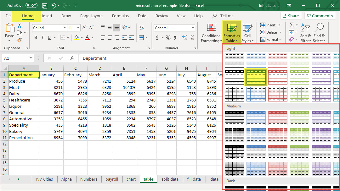
2. Select Home > Format as Table.
3. Choose a style for your table.
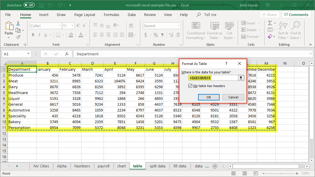
4. In the Format as Table dialog box, set your cell range.
5. Mark if your table has headers.
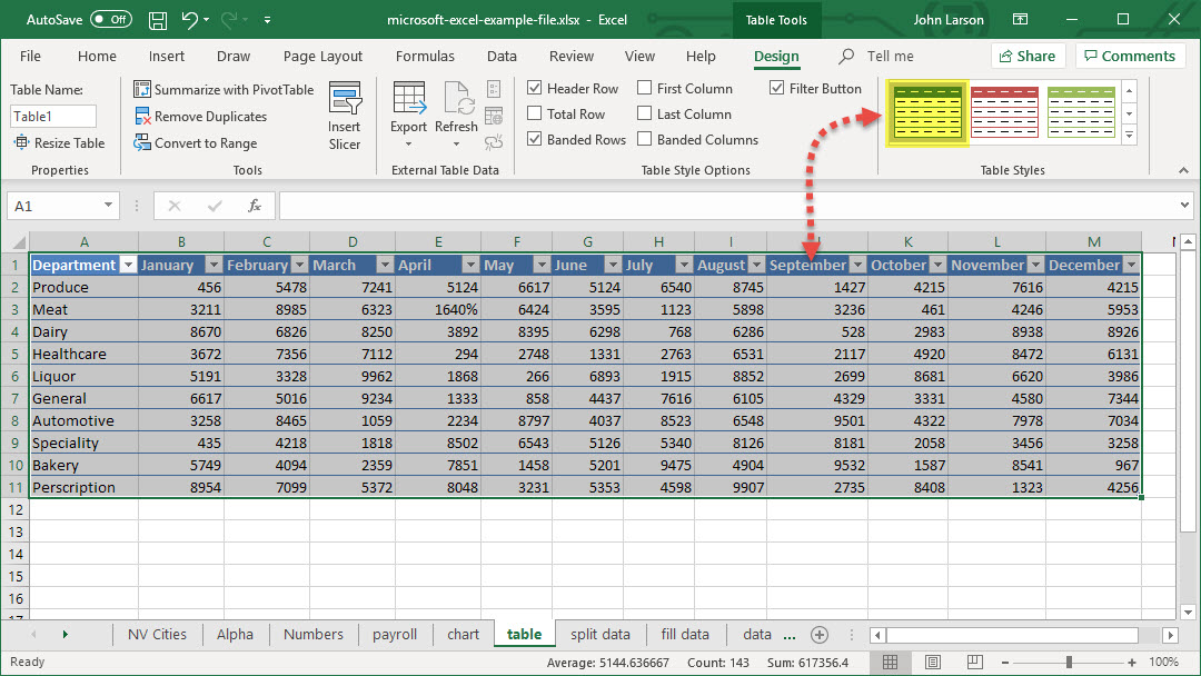
6. Select OK.
Sort Data in a Table
Sorting is one of the most common tools for data management. In Excel, you can sort your table by one or more columns, by ascending or descending order, or by doing a custom sort.
Before sorting a table
1. Make sure that there are no empty rows or columns in the table.
2. Get table headers into one row across the top.
3. Make sure there is at least one empty column between the table you want to sort, and other information on the worksheet not in that table.
Sort the table
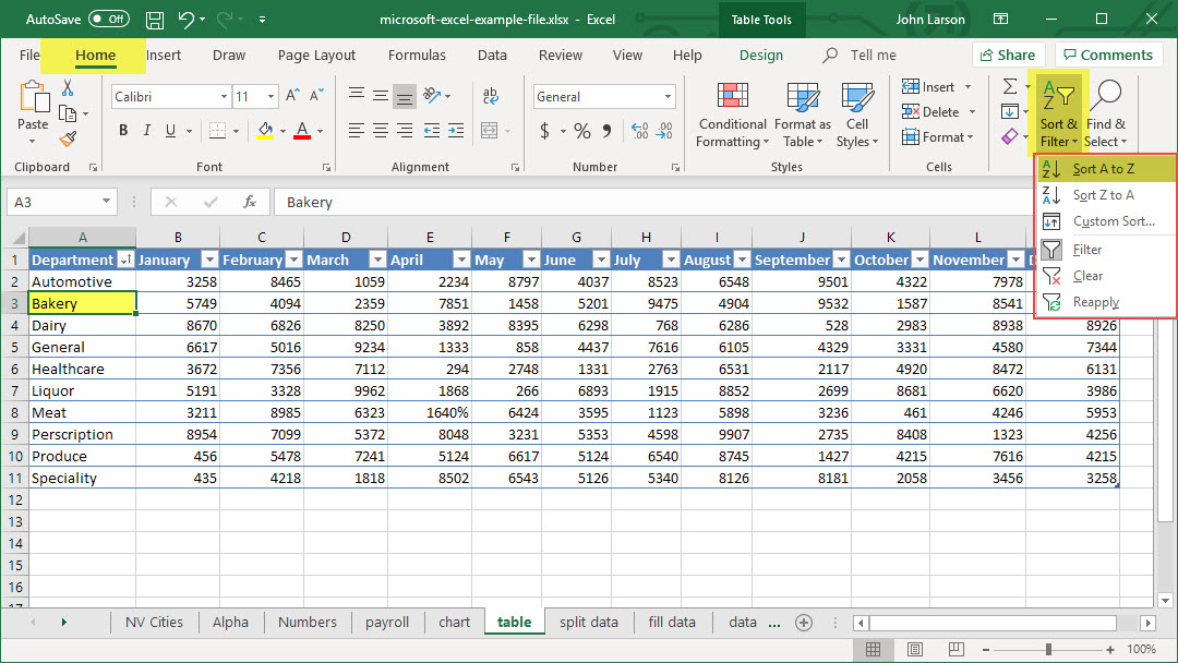
1. Select a cell within the data.
2. Select Home > Sort & Filter.
Or, select Data > Sort.
3. Select an option:
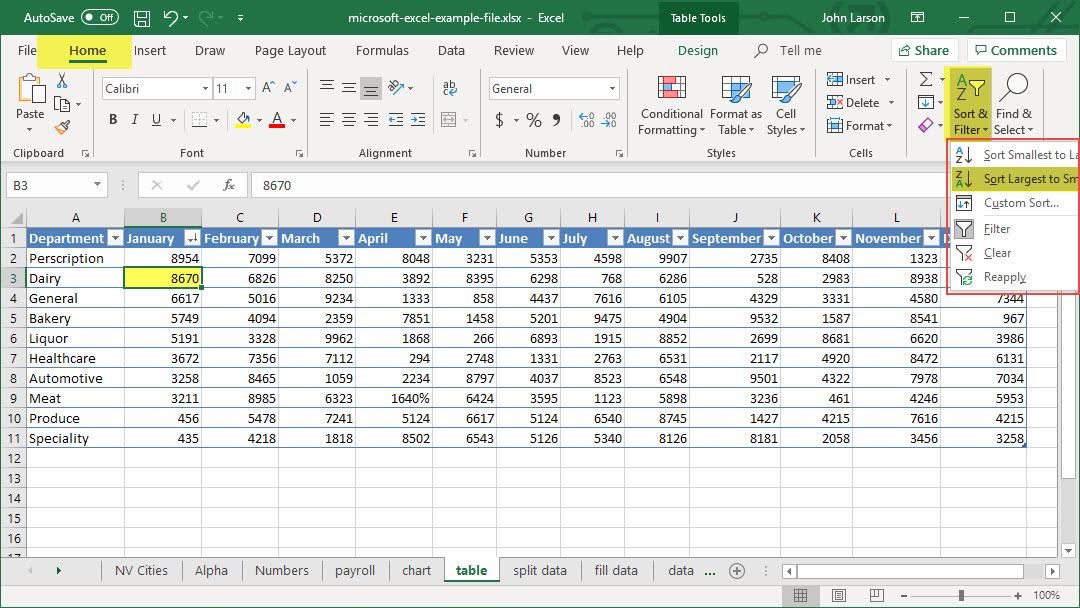
Sort A to Z – sorts the selected column in an ascending order.
Sort Z to A – sorts the selected column in a descending order.
Custom Sort – sorts data in multiple columns by applying different sort criteria.
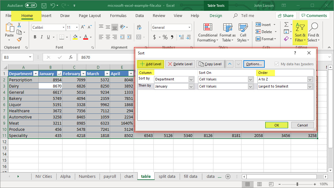
Here’s how to do a custom sort:
a. Select Custom Sort.
b. Select Add Level.
c. For Column, select the column you want to “Sort by” from the drop-down, and then select the second column “Then by” you want to sort. For example, Sort by Department and Then by Status.
d. For Sort On, select Values.
e. For Order, select an option, like A to Z, Smallest to Largest, or Largest to Smallest.
f. For each additional column that you want to sort by, repeat steps 2-5.
Note: To delete a level, select Delete Level.
g. Check the My data has headers checkbox, if your data has a header row.
h. Select OK.
Filter Data in a Range or Table
Use AutoFilter or built-in comparison operators like “greater than” and “top 10” in Excel to show the data you want and hide the rest. Once you filter data in a range of cells or table, you can either reapply a filter to get up-to-date results, or clear a filter to redisplay all of the data.
Use filters to temporarily hide some of the data in a table, so you can focus on the data you want to see.
Filter a range of data
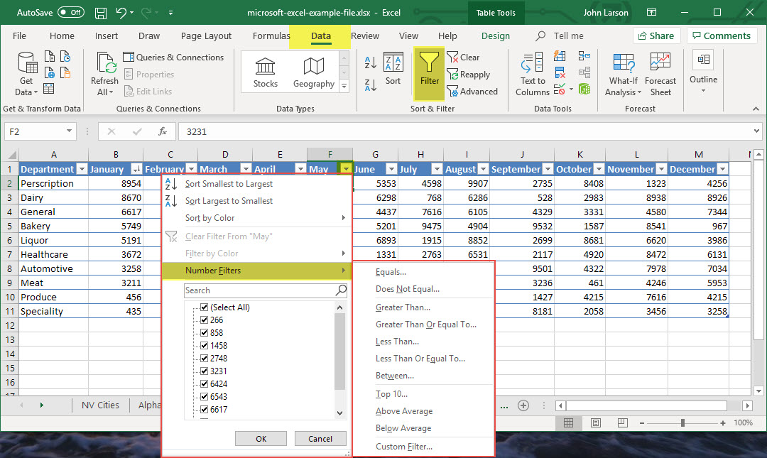
1. Select any cell within the range.
2. Select Data > Filter.
3. Select the column header arrow Filter arrow .
4. Select Text Filters or Number Filters, and then select a comparison, like Between.
5. Enter the filter criteria and select OK.
Filter data in a table
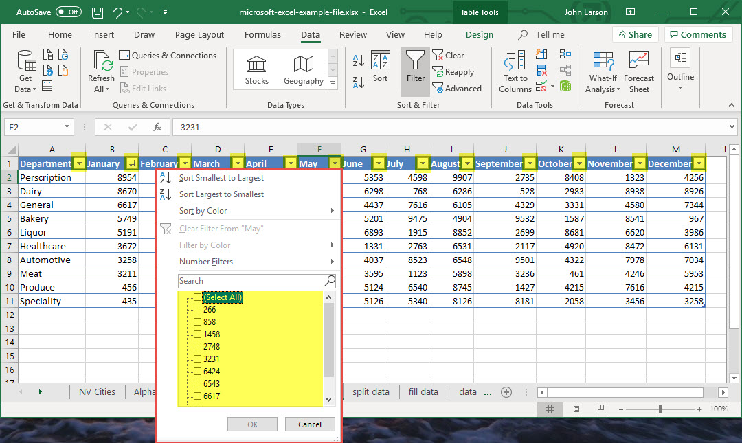
When you put your data in a table, filter controls are automatically added to the table headers.
1. Select the column header filter drop-down arrow for the column you want to filter.
2. Uncheck (Select All) and select the boxes you want to show.
3. Click OK.
The column header arrow filter drop-down arrow changes to an applied Filter icon. Select this icon to change or clear the filter.
Total the Data in an Excel Table
You can quickly total data in an Excel table by enabling the Total Row option, and then use one of several functions that are provided in a drop-down list for each table column. The Total Row default selections use SUBTOTAL functions, which allow you to include or ignore hidden table rows, however you can also use other functions.
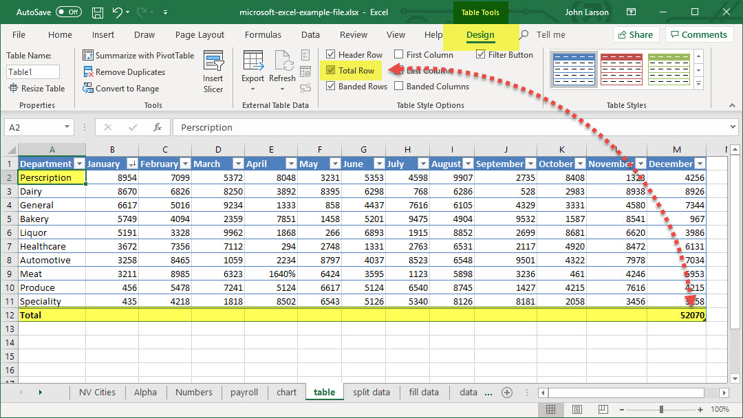
1. Click anywhere inside the table.
2. Go to Table Tools > Design, and select the check box for Total Row. On a Mac go to Table > Total Row.
3. The Total Row is inserted at the bottom of your table.
Note: If you apply formulas to a total row, then toggle the total row off and on, Excel will remember your formulas. In the previous example, we had already applied the SUM function to the total row. When you apply a total row for the first time, the cells will be empty.
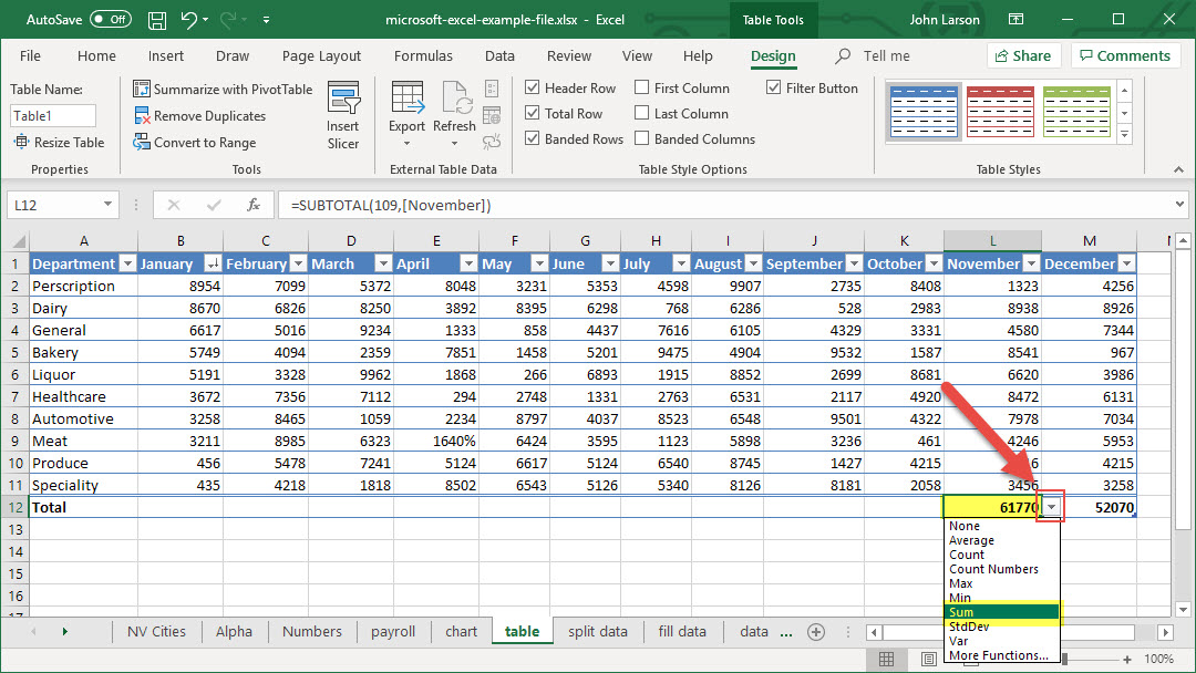
4. Select the column you want to total, then select an option from the drop-down list. In this case, we applied the SUM function to each column:
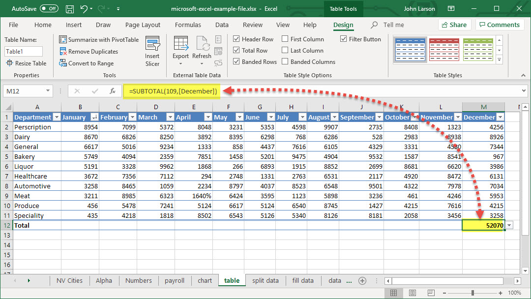
You’ll see that Excel created the following formula: =SUBTOTAL(109,[December]). This is a SUBTOTAL function for SUM, and it is also a Structured Reference formula, which is exclusive to Excel tables.
You can also apply a different function to the total value, by selecting the More Functions option or writing your own.
Note: If you want to copy a total row formula to an adjacent cell in the total row, drag the formula across using the fill handle. This will update the column references accordingly and display the correct value. If you copy and paste a formula in the total row, it will not update the column references as you copy across, and will result in inaccurate values.
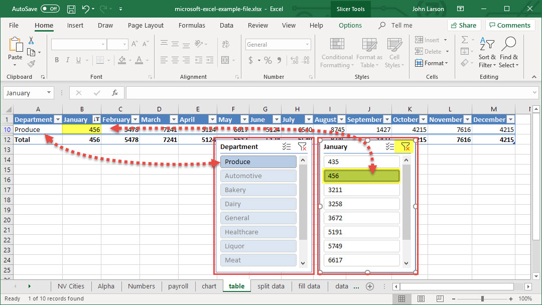
Use Slicers to Filter Data
Slicers provide buttons that you can click to filter table data, or PivotTable data. In addition to quick filtering, slicers also indicate the current filtering state, which makes it easy to understand what exactly is shown in a filtered PivotTable.
When you select an item, that item is included in the filter and the data for that item will be displayed in the report. For example, when you select Callahan in the Salespersons field, only data that includes Callahan in that field are displayed.
Use a slicer to filter data
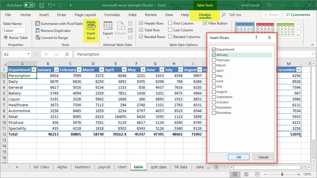
1. Click anywhere in the table.
2. Select Insert > Slicer ![]() .
.
3. Select the fields you’d like to filter.
4. Select OK and adjust your slicer preferences, such as Columns, under Options.
Note: To select more than one item, hold Ctrl, and then select the items that you want to show. Select and hold the corner of a slicer to adjust and resize it.
5. Select Clear Filter Delete ![]() to clear the slicer filter.
to clear the slicer filter.
Convert data into a table
1. There are four ways to convert data into a table:
Note: In order to use a slicer, you must convert your data into a table first.
- Press Ctrl + T.
- Press Ctrl + l.
- Select Home > Format as Table.
- Select Insert > Table.
2. Select OK.