Share your Excel workbook with others
Share a workbook with others, right within Excel. You can let them edit the workbook or just view it.
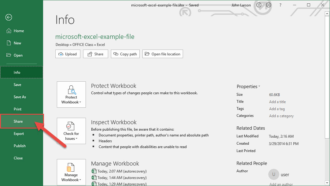
1. Select Share.
2. Select permissions and then Apply.
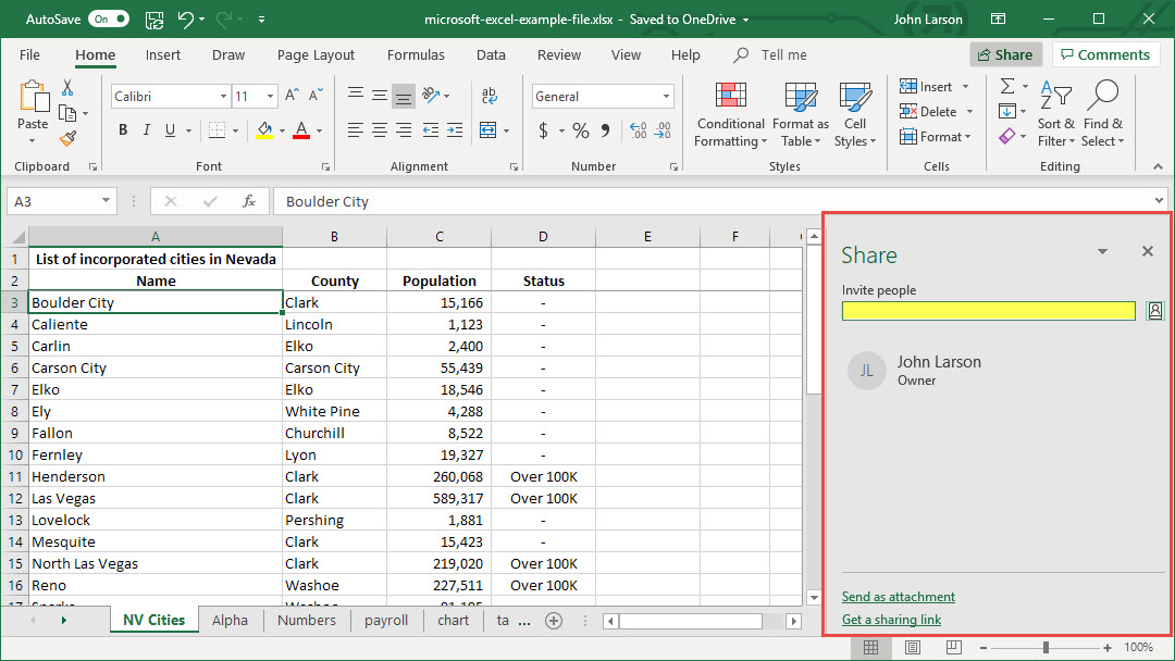
3. Add people.
4. Type a message if you like.
5. Select Send.
Annotate a worksheet by using comments
Add comments to cells to explain what the cells contain.
Add a comment

1. Right-click a cell and click Insert Comment.

2. In the comment box, type your comment.
3. Click outside the comment box.
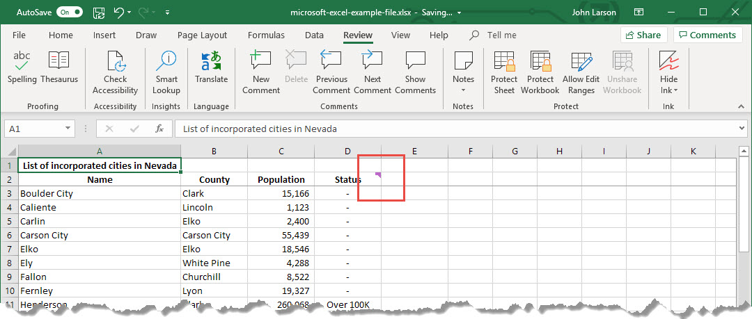
The comment box disappears, but a red comment indicator remains. To see the comment, hover over the cell.
Tip: To format your comment, highlight the text you want to change, right-click on the comment, and choose Format Comment.
Review comments
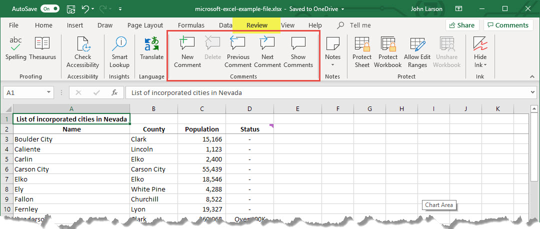
Select the Review tab, and click Next or Previous to see each comment in sequence.
See all comments at once

Select Review > Show All Comments to show or hide comments.
You may need to move or resize overlapping comments.
Note: Select Review > Show/Hide Comment to show or hide individual comments.
Reply to a comment
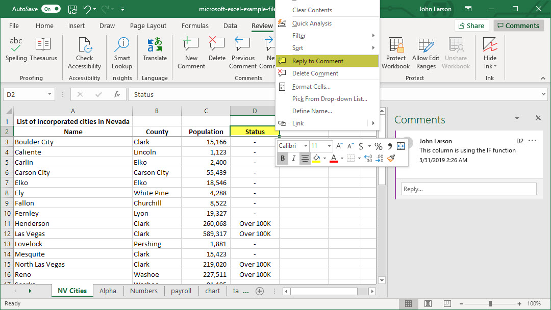
Right-click on the cell with the comment, select “Replay to Comment” and type the response in the “Replay” frame.
Delete a comment
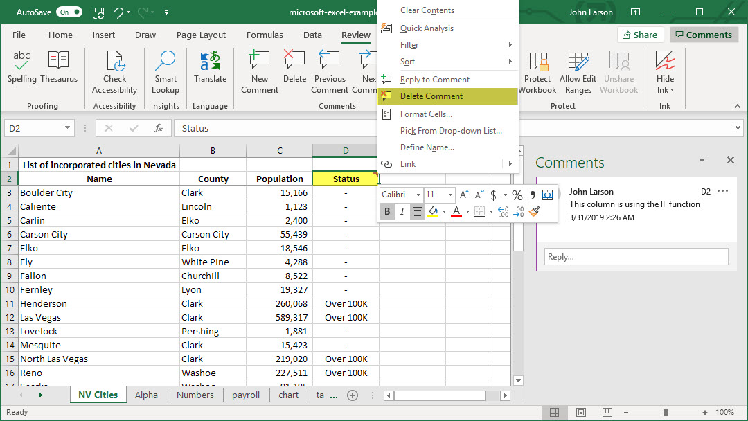
Right-click on the cell with the comment and select “Delete Comment” from the menu.
Collaborate on Excel workbooks at the same time with co-authoring
You and your colleagues can open and work on the same Excel workbook. This is called co-authoring. When you co-author, you can see each other’s changes quickly — in a matter of seconds. And with certain versions of Excel, you’ll see other people’s selections in different colors. If you’re using a version of Excel that supports co-authoring, you select Share in the upper-right corner, type email addresses, and then choose a cloud location.
Note: This feature is only available if you have an Office 365 subscription.
Steps
To co-author in Excel for Windows desktops, you need to make sure certain things are set up before you start. After that, it just takes about four steps to co-author with other people.
What you need to co-author
- You need an Office 365 subscription.
- You need the latest version of Excel for Office 365 installed. Please note that if you have a work or school account, you might not have a version of Office that supports co-authoring yet. This might be because your administrator hasn’t provided the latest version to install.
- You need to sign in to Office with your subscription account.
- You need to use Excel Workbooks in .xlsx, .xlsm, or .xlsb files. If your file isn’t in this format, open the file and then click File > Save As > Browse > Save as type. Change the format to Excel Workbook (*.xlsx). Please note that co-authoring does not support the Strict Open XML Spreadsheet format.
Step 1: Upload the workbook
Using a web browser, upload or create a new workbook on OneDrive, OneDrive for Business, or a SharePoint Online library. Please note that SharePoint On-Premises sites (sites that are not hosted by Microsoft), do not support co-authoring.
Step 2: Share it
1. If you uploaded the file, click the filename to open it. The workbook will open in a new tab in your web browser.
2. Click the Edit in Excel button. If you don’t have this button, click Edit in Browser, and then click Edit in Excel after the page reloads.
3. If you are prompted to choose a version of Excel, click Microsoft Excel.
4. When the file opens in the Excel program, you may see a yellow bar which says the file is in Protected View. Click the Enable Editing button if that’s the case.
5. Click Share in the upper-right.
6. Type email addresses in the Invite people box, and separate each with a semicolon. Make sure to also select Can edit. When you’re done, click the Share button.
Note: If you want to send the link yourself, don’t click the Share button. Instead, click Get a sharing link at the bottom of the pane.
7. If you clicked the Share button in the previous step, email messages will be sent to each person. The message will come from your email address. You will also receive a copy of the message, just so you know what it looks like.
Step 3: Other people can open it
If you clicked the Share button, people will receive an email message inviting them to open the file. They can click the link to open the workbook. A web browser will open, and the workbook will open in Excel Online. If they want to use an Excel app to co-author, they can click Edit Workbook > Edit in Excel. However, they’ll need a version of the Excel app that supports co-authoring. Excel for Android, Excel for iOS, Excel Mobile, and Excel for Office 365 subscribers are the versions that currently support co-authoring. If they don’t have a supported version, they can click Edit Workbook > Edit in Browser to edit the file.
Note: If they’re using the latest version of Excel, PowerPoint, or Word there’s an easier way: They can click File > Open and select Shared with Me.
Step 4: Co-author with others
With the file still open in Excel, make sure that AutoSave is on in the upper-left corner. When others eventually open the file, you’ll be co-authoring together. You know you’re co-authoring if you see pictures of people in the upper-right of the Excel window. (You may also see their initials or a “G” which stands for guest.)
Co-authoring tips:
- You might see other people’s selections in different colors. This happens if they are using Excel for Office 365 subscribers, Excel Online, Excel for Android, Excel Mobile, or Excel for iOS. If they’re using another version you won’t see their selections, but their changes will appear as they are working.
- If you see other people’s selections in different colors, they’ll show up as blue, purple, and so on. However, your selection will always be green. And on other people’s screens, their own selections will be green as well. If you lose track of who’s who, rest your cursor over the selection, and the person’s name will be revealed. If you want to jump to where someone is working, click their picture or initials, and then click the Go to option.
See files others have shared with you
The Shared (on Mac and iOS) or Shared with me (on Android, Windows Mobile or Windows Desktop) view lets you see the files others have shared with you. After you’re invited into the document, that document will automatically appear in the Shared or Shared with Me list. Office will try to show you more relevant shared documents at the top of the list.
This feature is only available if you have an Office 365 subscription. If you are an Office 365 subscriber, make sure you have the latest version of Office.
Notes:
- You will need to sign into Office with a Microsoft account or a Work or school account to see documents shared with you.
- Shared with Me shows only documents from OneDrive – Personal, OneDrive for Business and SharePoint Online.
- If someone who shares a file with you sets your permission level to “edit,” you’ll be able to share the file too.
To see the files that others have shared with you, go to File > Open > Shared with me.
Lock or unlock specific areas of a protected worksheet
By default, protecting a worksheet locks all cells so none of them are editable. To enable some cell editing, while leaving other cells locked, it’s possible to unlock all the cells. You can lock only specific cells and ranges before you protect the worksheet and, optionally, enable specific users to edit only in specific ranges of a protected sheet.
Lock only specific cells and ranges in a protected worksheet
1. If the worksheet is protected, do the following:
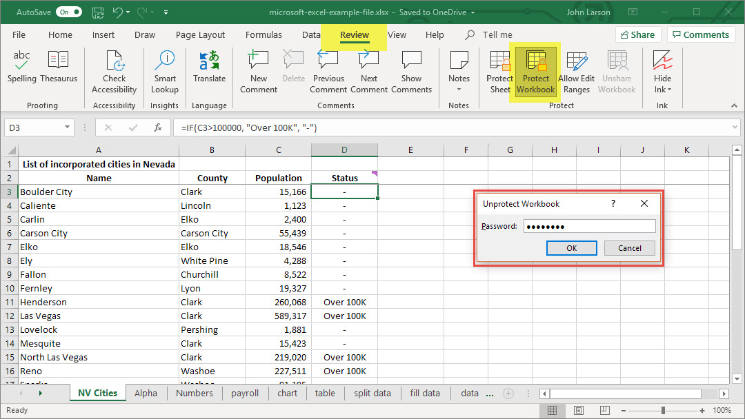
a. On the Review tab, click Unprotect Sheet (in the Changes group).
Click the Protect Sheet button to Unprotect Sheet when a worksheet is protected.
b. If prompted, enter the password to unprotect the worksheet.
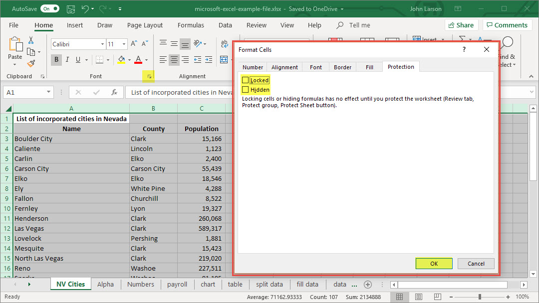
2. Select the whole worksheet by clicking the Select All button.
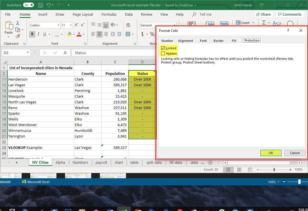
3. On the Home tab, click the Format Cell Font popup launcher. You can also press Ctrl+Shift+F or Ctrl+1.
4. In the Format Cells popup, in the Protection tab, uncheck the Locked box and then click OK.
This unlocks all the cells on the worksheet when you protect the worksheet. Now, you can choose the cells you specifically want to lock.
5. On the worksheet, select just the cells that you want to lock.
6. Bring up the Format Cells popup window again (Ctrl+Shift+F).
7. This time, on the Protection tab, check the Locked box and then click OK.
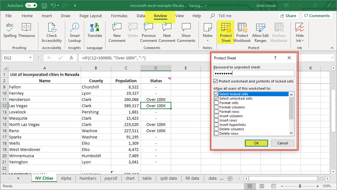
8. On the Review tab, click Protect Sheet.
9. In the Allow all users of this worksheet to list, choose the elements that you want users to be able to change.
More information about worksheet elements
| Clear this check box | To prevent users from |
| Select locked cells | Moving the pointer to cells for which the Locked check box is selected on the Protection tab of the Format Cells dialog box. By default, users are allowed to select locked cells. |
| Select unlocked cells | Moving the pointer to cells for which the Locked check box is cleared on the Protection tab of the Format Cells dialog box. By default, users can select unlocked cells, and they can press the TAB key to move between the unlocked cells on a protected worksheet. |
| Format cells | Changing any of the options in the Format Cells or Conditional Formatting dialog boxes. If you applied conditional formats before you protected the worksheet, the formatting continues to change when a user enters a value that satisfies a different condition. |
| Format columns | Using any of the column formatting commands, including changing column width or hiding columns (Home tab, Cells group, Format button). |
| Format rows | Using any of the row formatting commands, including changing row height or hiding rows (Home tab, Cells group, Format button). |
| Insert columns | Inserting columns. |
| Insert rows | Inserting rows. |
| Insert hyperlinks | Inserting new hyperlinks, even in unlocked cells. |
| Delete columns | Deleting columns.
If Delete columns is protected and Insert columns is not also protected, a user can insert columns that he or she cannot delete. |
| Delete rows | Deleting rows.
If Delete rows is protected and Insert rows is not also protected, a user can insert rows that he or she cannot delete. |
| Sort | Using any commands to sort data (Data tab, Sort & Filter group).
Users can’t sort ranges that contain locked cells on a protected worksheet, regardless of this setting. |
| Use AutoFilter | Using the drop-down arrows to change the filter on ranges when AutoFilters are applied.
Users cannot apply or remove AutoFilters on a protected worksheet, regardless of this setting. |
| Use PivotTable reports | Formatting, changing the layout, refreshing, or otherwise modifying PivotTable reports, or creating new reports. |
| Edit objects | Doing any of the following:
|
| Edit scenarios | Viewing scenarios that you have hidden, making changes to scenarios that you have prevented changes to, and deleting these scenarios. Users can change the values in the changing cells, if the cells are not protected, and add new scenarios. |
Chart sheet elements
| Select this check box | To prevent users from |
| Contents | Making changes to items that are part of the chart, such as data series, axes, and legends. The chart continues to reflect changes made to its source data. |
| Objects | Making changes to graphic objects — including shapes, text boxes, and controls — unless you unlock the objects before you protect the chart sheet. |
10. In the Password to unprotect sheet box, type a password for the sheet, click OK, and then retype the password to confirm it.
- The password is optional. If you do not supply a password, any user can unprotect the sheet and change the protected elements.
- Make sure that you choose a password that is easy to remember, because if you lose the password, you won’t have access to the protected elements on the worksheet.
Protect an Excel file
To prevent others from accessing data in your Excel files, protect your Excel file with a password.
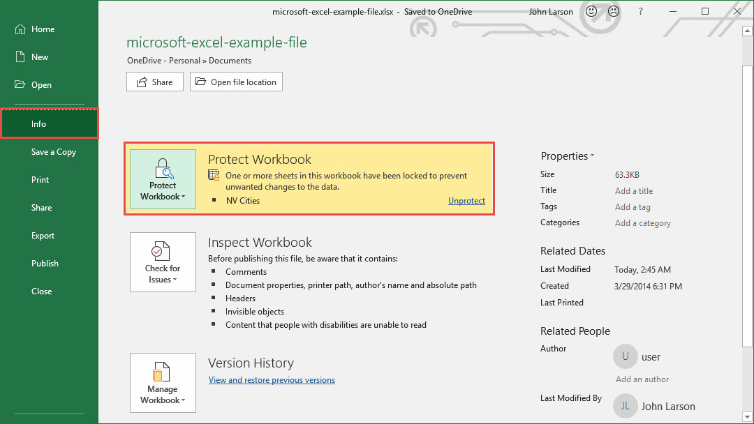
1. Select File > Info.
2. Select the Protect Workbook box and choose Encrypt with Password.
3. Enter a password in the Password box, and then select OK.
4. Confirm the password in the Reenter Password box, and then select OK.
Warning:
- Microsoft cannot retrieve forgotten passwords, so be sure that your password is especially memorable.
- There are no restrictions on the passwords you use concerning length, characters, or numbers, but passwords are case-sensitive.
- It’s not always secure to distribute password-protected files that contain sensitive information such as credit card numbers.
- Be cautious when sharing files or passwords with other users. You still run the risk of passwords falling into the hands of unintended users. Remember that locking a file with a password does not necessarily protect your file from malicious intent.
Save or convert to PDF
Use the Office programs to save or convert your files to PDFs, so that you can share them or print them using commercial printers. And you won’t need any other software or add-ins.
Use the PDF format for files that you want to look the same on most computers, have a smaller font size, and comply with an industry-standard – like resumes, legal documents, newsletters, or files only intended to be read or printed professionally.
Save or convert to PDF
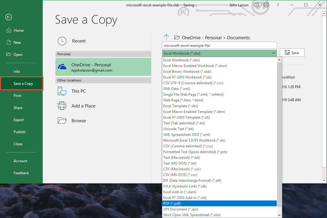
1. Click File > Save As.
To see the Save As dialog box in Excel 2013 or Excel 2016, you have to choose a location and folder.
2. In the File Name box, enter a name for the file if you haven’t already.
3. In the Save as type list, click PDF (*.pdf).
To open in the selected format after saving, select the Open file after publishing check box.
If the document requires high print quality, click Standard (publishing online and printing).
If file size is more important than print quality, click Minimum size (publishing online).
4. Click Options to set the page to be printed, to choose whether markup should be printed, and to select output options. Click OK when finished.
5. Click Save.
Notes:
- To view a PDF file, you must have a PDF reader installed on your computer such as the Acrobat Reader, available from Adobe Systems.
- This procedure also applies to Microsoft Excel Starter 2010.
- You can’t save Power View sheets as PDF files.