- Insert or Delete Cells, Rows, or Columns
- Select Cell Contents
- Resize a Table, Column, or Row
- Freeze Panes to Lock Rows or Columns
- Hide or Show Rows or Columns
Insert or Delete Cells, Rows, or Columns
Insert and delete rows, columns, and cells to organize your worksheet better.
Note: Microsoft Excel has the following column and row limits: 16,384 columns wide by 1,048,576 rows tall.
Insert or delete a column
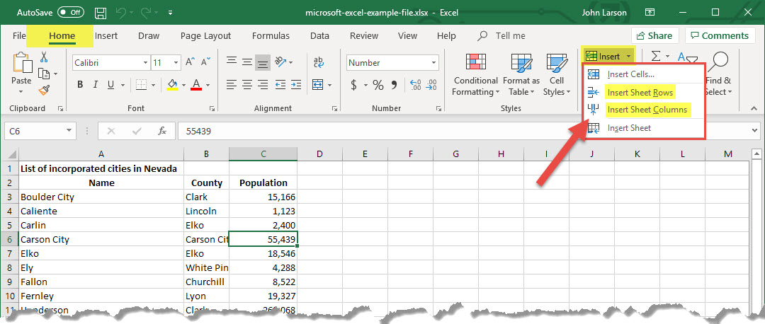
To insert a column, select the column, select Home > Insert > Insert Sheet Columns.
To delete a column, select the column, select Home > Insert > Delete Sheet Columns.
Or, right-click the top of the column, and then select Insert or Delete.
Insert or delete a row
To insert a row, select the row, select Home > Insert > Insert Sheet Rows.
To delete a row, select the row, select Home > Insert > Delete Sheet Rows.
Or, right-click the selected row, and then select Insert or Delete.
Insert or delete a cell
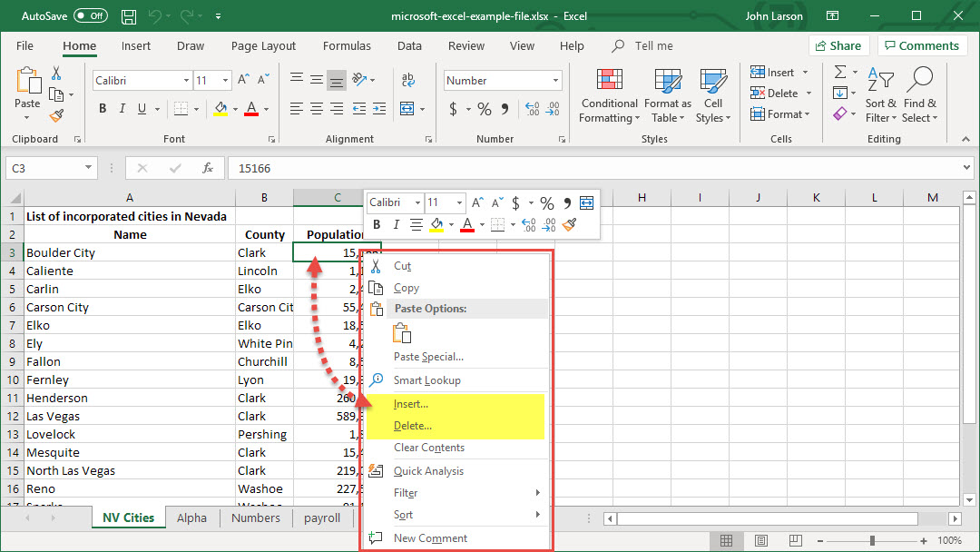
Select one or more cells. Right-click and select Insert.
From the Insert box, select a row, column or cell to insert.
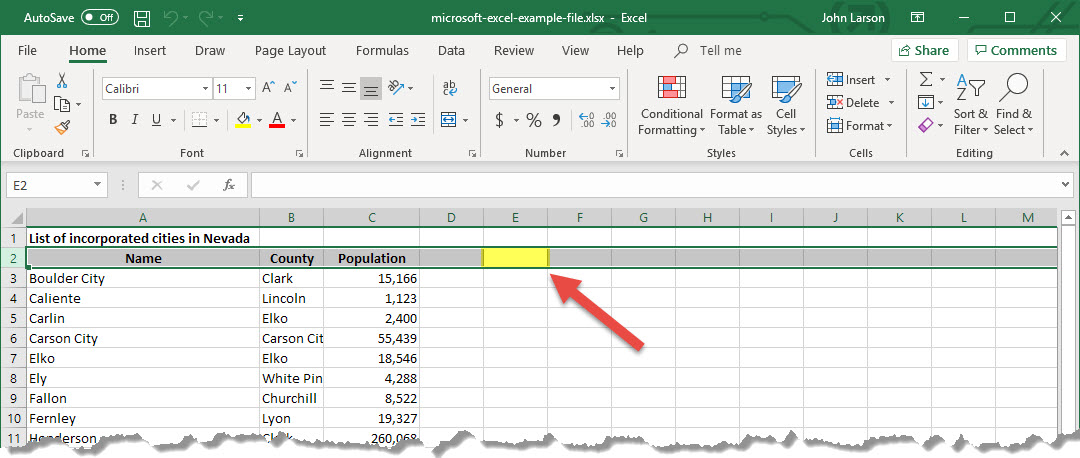
Selecting Cell Content
You can select the cell contents of one or more cells, rows, and/or columns.
Note: If a worksheet has been protected, you might not be able to select cells or their contents on a worksheet.
Selecting one or more cells
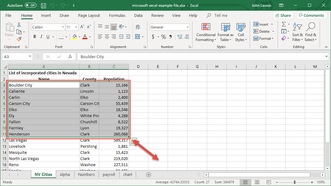
Click on a cell to select it. Or use the keyboard to navigate to it and select it.
To select a range, select a cell, then hold the right bottom edge and drag over the cell range. Or use the Shift + arrow keys to select the range.
To select non-adjacent cells and cell ranges, hold Ctrl and select the cells.
Selecting one or more rows and columns
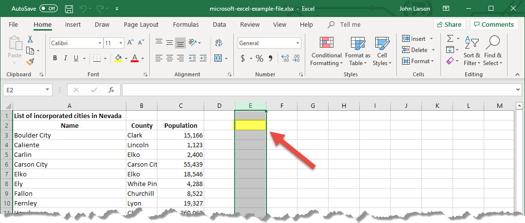
Select the letter at the top to select the entire column. Or click on any cell in the column and then press Ctrl+Space.
Select the row number to select the entire row. Or click on any cell in the row and then press Shift+Space.
To select non-adjacent rows or columns, hold Ctrl and select the row or column numbers.
Selecting a table, list, or worksheet
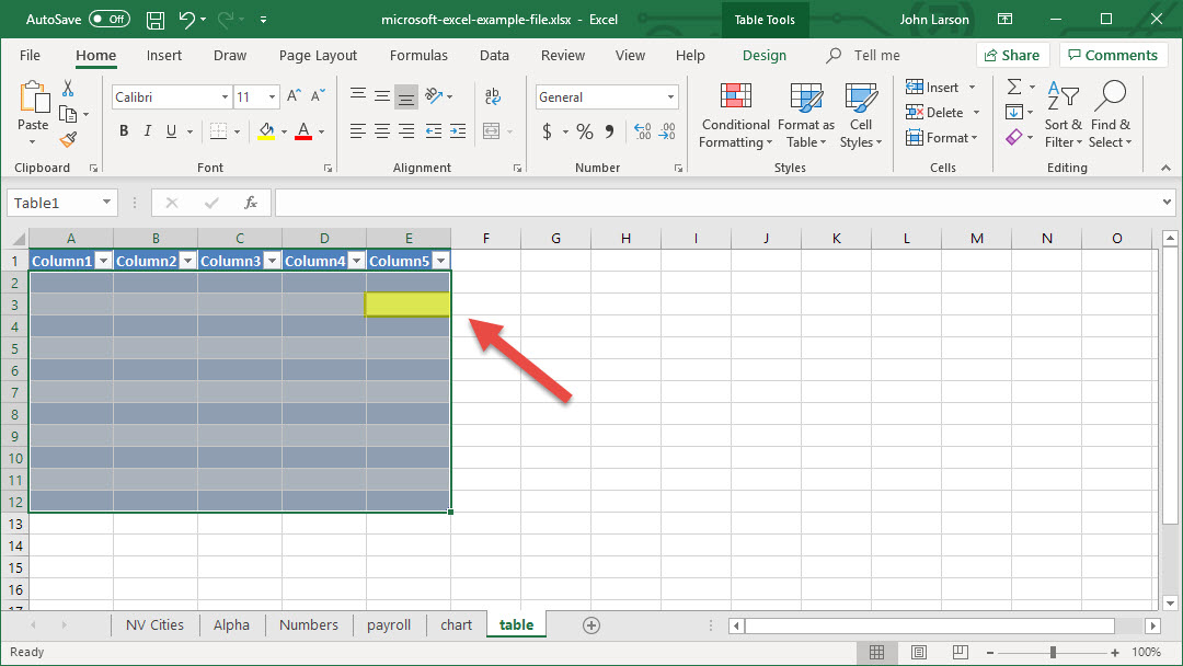
To select a list or table, select a cell in the list or table and press Ctrl+A.
To select the entire worksheet, press Ctrl+A+A. Or use the Select All button at the top left corner.
Resize a Table, Column, or Row
You can manually adjust the column width or row height or automatically resize columns and rows to fit the data.
Note: The boundary is the line between cells, columns, and rows. If a column is too narrow to display the data, you will see ### in the cell.
Resize rows
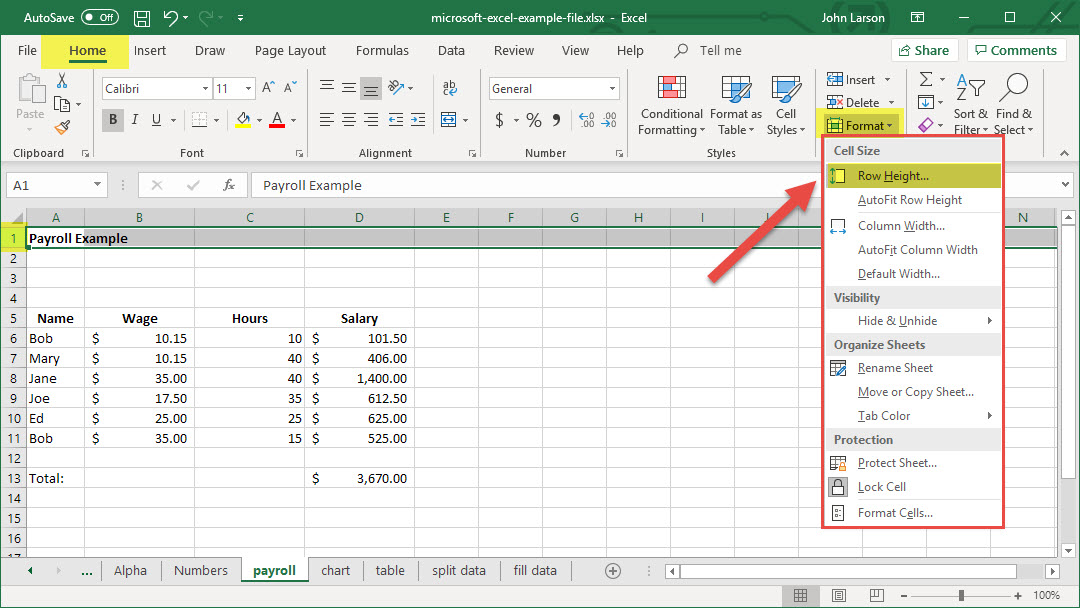
1. Select a row or a range of rows.
2. Select Format > Row Height.
3. Type the row height and select OK.
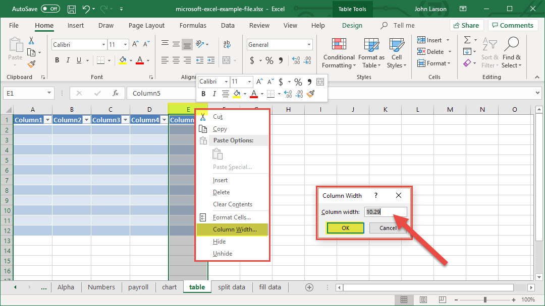
Resize columns – Option 1
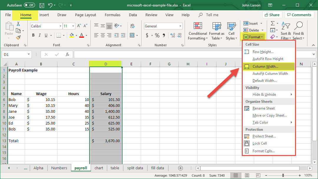
1. Select a column or a range of columns.
2. Select Format > Column Width.
3. Type the column width and select OK.
Resize columns – Option 2
1. Select a column or a range of columns.
2. Select Format > Column Width.
3. Type the column width and select OK.
Automatically resize all columns and rows to fit the data
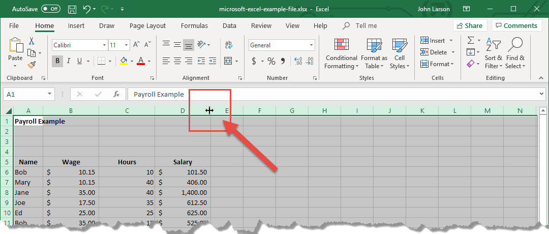
1. Select the Select All button at the top of the worksheet, to select all columns and rows.
2. Double-click a boundary. All columns or rows resize to fit the data.
Freeze Panes to Lock Rows or Columns
To keep an area of a worksheet visible while you scroll to another area of the worksheet, go to the View tab, where you can Freeze Panes to lock specific rows and columns in place, or you can Split panes to create separate windows of the same worksheet.
Freeze rows or columns
Freeze the first column
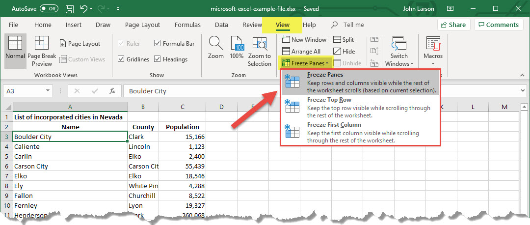
Select View > Freeze Panes > Freeze First Column.
The faint line that appears between Columns A and B shows that the first column is frozen.
Freeze the first two columns
1. Select the third column.
2. Select View > Freeze Panes > Freeze Panes.
Freeze columns and rows
1. Select the cell below the rows and to the right of the columns you want to keep visible when you scroll.
2. Select View > Freeze Panes > Freeze Panes.
Unfreeze rows or columns
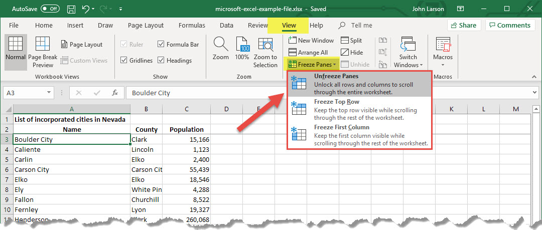
On the View tab > Window > Unfreeze Panes.
Note: If you don’t see the View tab, it’s likely that you are using Excel Starter. Not all features are supported in Excel Starter.
Hide or Show Rows or Columns
Hide or unhide columns in your spreadsheet to show just the data that you need to see or print.
Hide columns
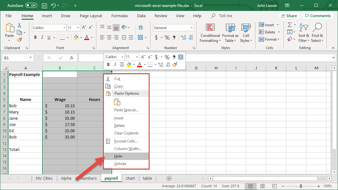
1. Select one or more columns, and then press Ctrl to select additional columns that aren’t adjacent.
2. Right-click the selected columns, and then select Hide.
Note: The double line between two columns is an indicator that you’ve hidden a column.
Unhide columns
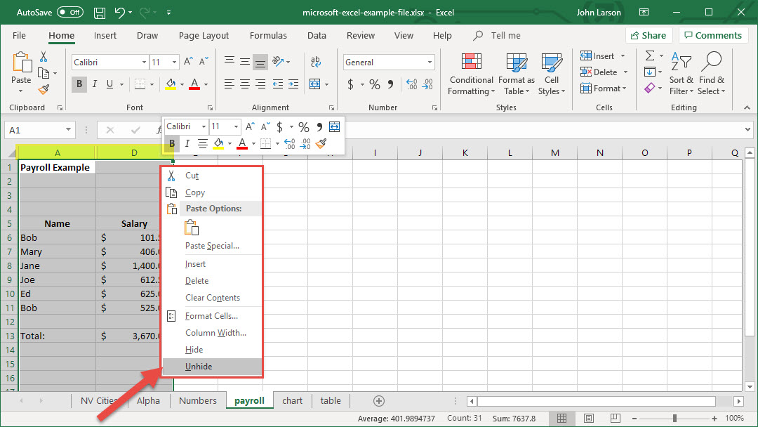
1. Select the adjacent columns for the hidden columns.
2. Right-click the selected columns, and then select Unhide or double-click the double line between the two columns where hidden columns exist.