Common Tasks for Excel Beginners
This section builds upon the foundational knowledge of cells, rows & columns, and formatting, and prepares you for using formulas and functions effectively. Here are some common Excel tasks you should learn:
Data Entry and Organization:
Data Manipulation:
- Combine Text from Two or More Cells
- Split Text into Different Columns
- Create a List of Sequential Data
Formatting and Analysis:
- Filter for Unique Values or Remove Duplicate Values
- Apply Data Validation to Cells
- Conditional Formatting
By mastering these common tasks, you’ll gain a solid foundation for using Excel for various purposes and be well-prepared to delve into more advanced features like formulas and functions.
Import or Export Text Files
There are two ways to import data from a text file with Excel: you can open it in Excel, or you can import it as an external data range. To export data from Excel to a text file, use the Save As command and change the file type from the drop-down menu.
There are two commonly used text file formats:
- Delimited text files (.txt), in which the TAB character (ASCII character code 009) typically separates each field of text.
- Comma-separated values text files (.csv), in which the comma character (,) typically separates each field of text.
You can change the separator character that is used in both delimited and .csv text files. This may be necessary to make sure that the import or export operation works the way that you want it to.
Note: You can import or export up to 1,048,576 rows and 16,384 columns.
Import a text file by opening it in Excel
You can open a text file that you created in another program as an Excel workbook by using the Open command. Opening a text file in Excel does not change the format of the file — you can see this in the Excel title bar, where the name of the file retains the text file name extension (for example, .txt or .csv).
1. Go to File > Open.
2. Select Text Files from the Open dialog box.
3. Locate and double-click the text file that you want to open.
- If the file is a text file (.txt), Excel starts the Import Text Wizard. When you are done with the steps, click Finish to complete the import operation.
- If the file is a .csv file, Excel automatically opens the text file and displays the data in a new workbook.
Note: When Excel opens a .csv file, it uses the current default data format settings to interpret how to import each column of data. If you want more flexibility in converting columns to different data formats, you can use the Import Text Wizard. For example, the format of a data column in the .csv file may be MDY, but Excel’s default data format is YMD, or you want to convert a column of numbers that contains leading zeros to text so you can preserve the leading zeros. To force Excel to run the Import Text Wizard, you can change the file name extension from .csv to .txt before you open it, or you can Import a text file by connecting to it.
Find or Replace Text and Numbers
Use the Find and Replace features in Excel to search for something in your workbook, such as a particular number or text string.
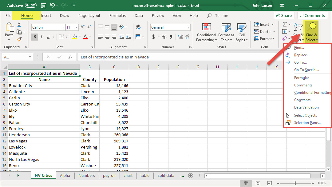
1. On the Home tab, in the Editing group, click Find & Select.
2. Do one of the following:
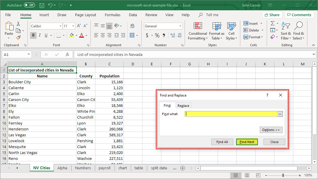
To find text or numbers, click Find.
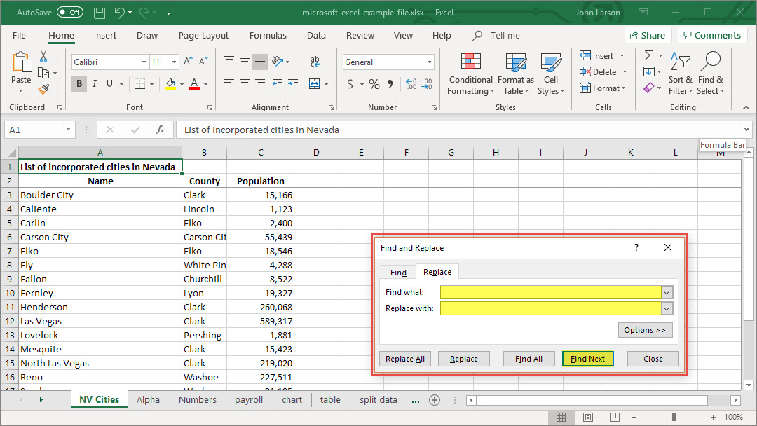
To find and replace text or numbers, click Replace.
3. In the Find box, type the text or numbers you want to search for, or click the arrow in the Find box, and then click a recent search in the list.
You can use wildcard characters, such as an asterisk (*) or a question mark (?), in your search criteria:
- Use the asterisk to find any string of characters. For example, s*d finds “sad” and “started”.
- Use the question mark to find any single character. For example, s?t finds “sat” and “set”.
Tip: You can find asterisks, question marks, and tilde characters (~) in worksheet data by preceding them with a tilde character in the Find what box. For example, to find data that contain “?”, you would type ~? as your search criteria.
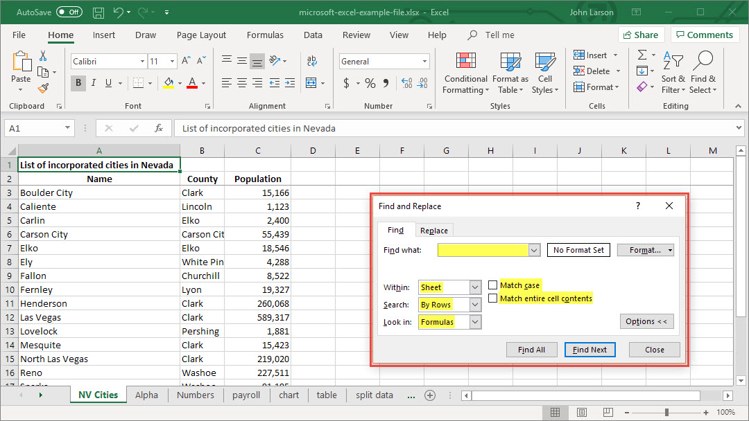
4. Click Options to further define your search if needed:
- To search for data in a worksheet or in an entire workbook, in the Within box, select Sheet or Workbook.
- To search for data in rows or columns, in the Search box, click By Rows or By Columns.
- To search for data with specific details, in the Look in box, click Formulas, Values, or Comments.
Note: Formulas, Values, Notes, and Comments are only available on the Find tab; only Formulas are available on the Replace tab.
- To search for case-sensitive data, select the Match case check box.
- To search for cells that contain just the characters that you typed in the Find what box, select the Match entire cell contents check box.
5. If you want to search for text or numbers with specific formatting, click Format, and then make your selections in the Find Format dialog box.
Tip: If you want to find cells that just match a specific format, you can delete any criteria in the Find box, and then select a specific cell format as an example. Click the arrow next to Format, click Choose Format From Cell, and then click the cell that has the formatting that you want to search for.
6. Do one of the following:
- To find text or numbers, click Find All or Find Next.
Tip: When you click Find All, every occurrence of the criteria that you are searching for will be listed, and clicking a specific occurrence in the list will make a cell active. You can sort the results of a Find All search by clicking a column heading.
- To replace text or numbers, type the replacement characters in the Replace with box (or leave this box blank to replace the characters with nothing), and then click Find or Find All.
Note: If the Replace with box is not available, click the Replace tab.
If needed, you can cancel a search in progress by pressing ESC.
7. To replace the highlighted occurrence or all occurrences of the found characters, click Replace or Replace All.
Tips:
- Microsoft Excel saves the formatting options you define. If you search the worksheet for data again and cannot find characters you know to be there, you may need to clear the formatting options from the previous search. In the Find and Replace dialog box, click the Find tab, and then click Options to display the formatting options. Click the arrow next to Format, and then click Clear Find Format.
- You can also use the SEARCH and FIND functions to find text or numbers on a worksheet.
Automatically Fill Rows or Columns
Unlike other Microsoft Office programs, Excel does not provide a button to number data automatically. But, you can easily add sequential numbers to rows of data by dragging the fill handle to fill a column with a series of numbers or by using the ROW function.
Tip: If you are looking for a more advanced auto-numbering system for your data, and Access is installed on your computer, you can import the Excel data to an Access database. In an Access database, you can create a field that automatically generates a unique number when you enter a new record in a table.
Fill a column with a series of numbers
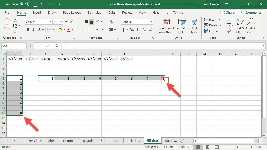
1. Select the first cell in the range that you want to fill.
2. Type the starting value for the series.
3. Type a value in the next cell to establish a pattern.
Tip: For example, if you want the series 1, 2, 3, 4, 5…, type 1 and 2 in the first two cells. If you want the series 2, 4, 6, 8…, type 2 and 4.
4. Select the cells that contain the starting values.
Note: In Excel 2013 and later, the Quick Analysis button is displayed by default when you select more than one cell containing data. You can ignore the button to complete this procedure.
5. Drag the fill handle ![]() across the range that you want to fill.
across the range that you want to fill.
Note: As you drag the fill handle across each cell, Excel displays a preview of the value. If you want a different pattern, drag the fill handle by holding down the right-click button, and then choose a pattern.
To fill in increasing order, drag down or to the right. To fill in decreasing order, drag up or to the left.
Note: These numbers are not automatically updated when you add, move, or remove rows. You can manually update the sequential numbering by selecting two numbers that are in the right sequence, and then dragging the fill handle to the end of the numbered range.
Use the ROW function to number rows
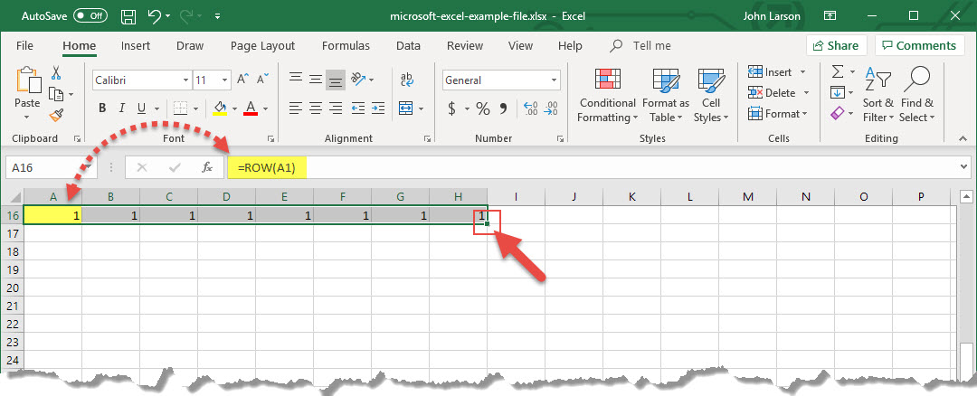
1. In the first cell of the range that you want to number, type =ROW(A1).
The ROW function returns the number of the row that you reference. For example, =ROW(A1) returns the number 1.
2. Drag the fill handle across the range that you want to fill.
- These numbers are updated when you sort them with your data. The sequence may be interrupted if you add, move, or delete rows. You can manually update the numbering by selecting two numbers that are in the right sequence, and then dragging the fill handle to the end of the numbered range.
- If you are using the ROW function, and you want the numbers to be inserted automatically as you add new rows of data, turn that range of data into an Excel table. All rows that are added at the end of the table are numbered in sequence.
To enter specific sequential number codes, such as purchase order numbers, you can use the ROW function together with the TEXT function. For example, to start a numbered list by using 000-001, you enter the formula =TEXT(ROW(A1),”000-000″) in the first cell of the range that you want to number, and then drag the fill handle to the end of the range.
Display or hide the fill handle
1. The fill handle displays by default, but you can turn it on or off.
In Excel 2010 and later, click the File tab, and then click Options.
In Excel 2007, click the Microsoft Office Button image, and then click Excel Options.
In the Advanced category, under Editing options, select or clear the Enable fill handle and cell drag-and-drop check box to display or hide the fill handle.
Note: To help prevent replacing existing data when you drag the fill handle, ensure the Alert before overwriting cells check box is selected. If you do not want Excel to display a message about overwriting cells, you can clear this check box.
Combine Text from Two or More Cells into One Cell
Excell offers multiple ways to join (concatenate) cell data. From simply combining cells to using functions that can handle a range of cells creating some interesting options for you to use.
Here are three techniques to join cell data:
1. Combine data with the Ampersand symbol (&)
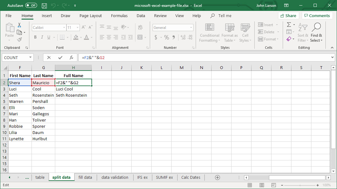
1. Select the cell where you want to put the combined data.
2. Type = and select the first cell you want to combine.
3. Type & and use quotation marks with a space enclosed.
4. Select the next cell you want to combine and press enter. An example formula might be =A2&” “&B2.
2. Combine data using the CONCAT function
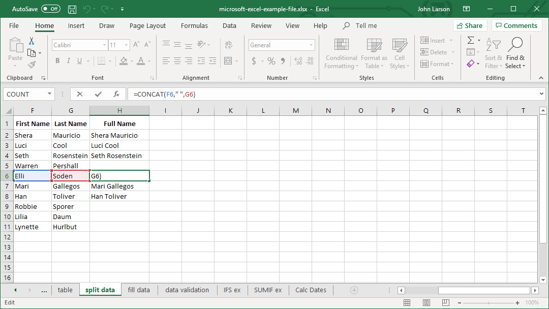
1. Select the cell where you want to put the combined data.
2. Type =CONCAT followed by the opening parenthesis “(“.
3. Select the cell you want to combine first.
Use commas to separate the cells you are combining and use quotation marks to add spaces, commas, or other text.
4. Close the formula with a parenthesis “)” and press Enter. An example formula might be =CONCAT(A2, ” Family”).
3. Combine data using the TEXTJOIN function
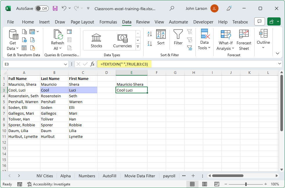
To join the first name (column B) and second name (column C) using the TEXTJOIN function, we would use a formula like this:
=TEXTJOIN(” “,TRUE,B2:C2)
The syntax for the TEXTJOIN function is as follows:
=TEXTJOIN(delimiter, ignore_empty, text1, [text2], …)
Arguments:
- delimiter: Separator between each text.
- ignore_empty: Whether to ignore empty cells or not.
- text1: First text value or range.
- text2: [optional] Second text value or range.
 ExcelJet offers summaries and examples for using both the TEXTJOIN and CONCAT functions. Their examples will illustrate the power these functions offer you as well as give you some creative ideas for using Excel.
Split Text into Different Columns
Convert Text to Columns Wizard
You can take the text in one cell and split it into multiple cells using the Convert Text to Columns wizard.
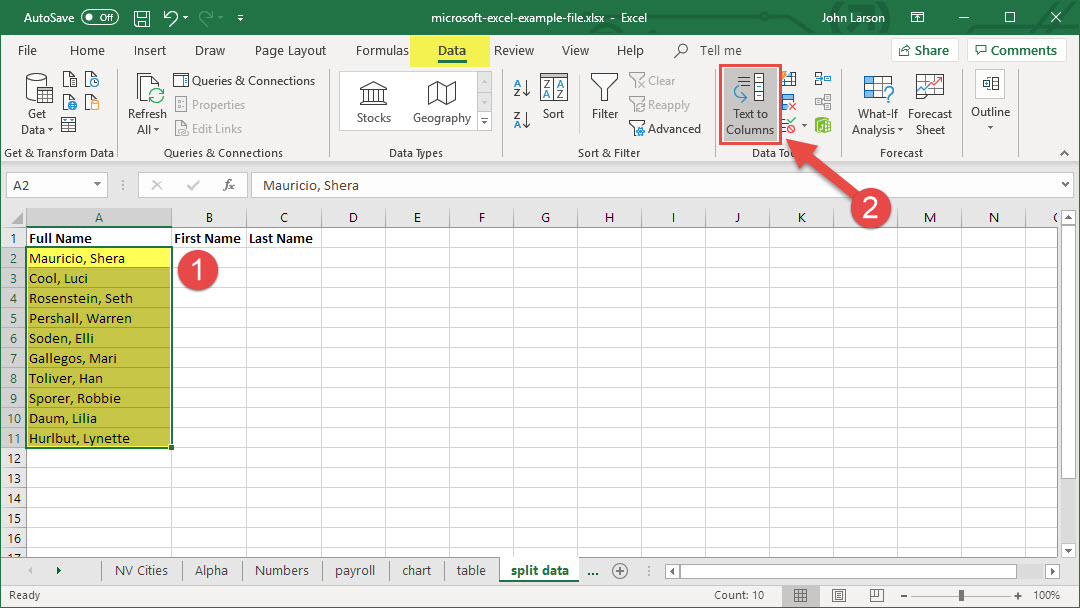
1. Select the cell or column that contains the text you want to split.
2. Select Data > Text to Columns.
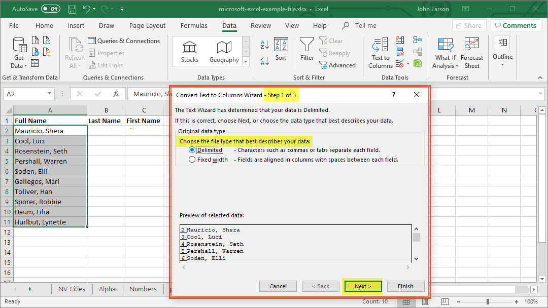
3. In the Convert Text to Columns Wizard, select Delimited > Next.
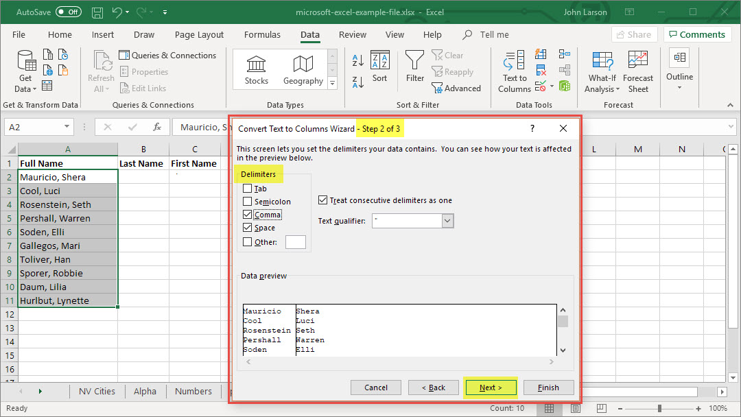
4. Select the Delimiters for your data. For example, Commas or Spaces. You can see a preview of your data in the Data preview window.
5. Select Next.
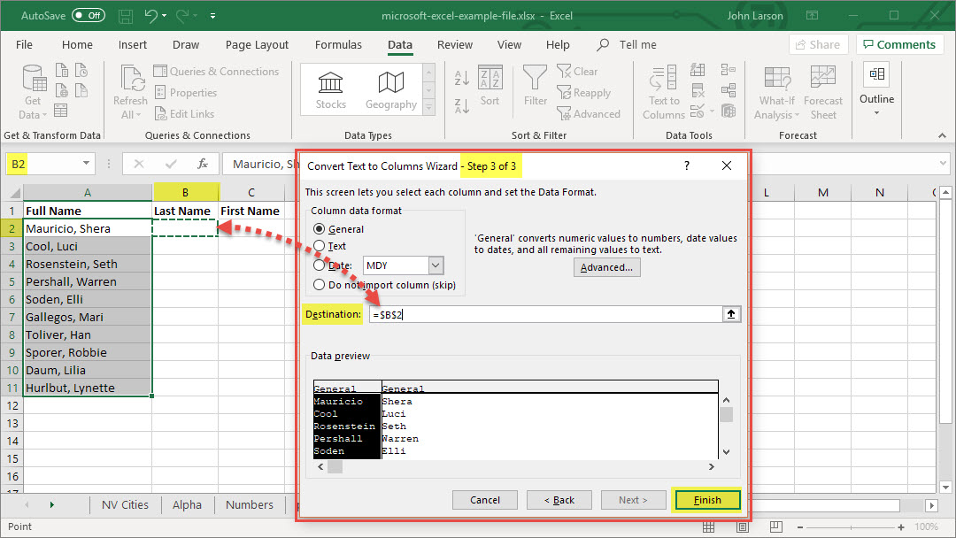
6. Select the Column data format or use what Excel chose for you.
7. Select the Destination, which is where you want the split data to appear on your worksheet.
8. Select Finish.
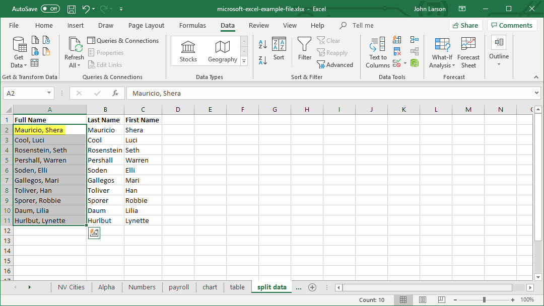
9. The contents from column A will be split into columns B and C.
Other Methods to Split Text
Excel also offers the TEXTBEFORE and TEXTAFTER functions to split cell data. The TEXTBEFORE function extracts all text before a defined delimiter (like a comma, dash, or any other defined character or characters), and the TEXTAFTER function extracts all text after a defined delimiter.
The syntax for the TEXTBEFORE function is as follows:
=TEXTBEFORE(text, delimiter, [instance_num], [match_mode], [match_end], [if_not_found] )
Arguments:
- text: The text you are searching within. Wildcard characters are not allowed. If text is an empty string, Excel returns empty text. Required.
- delimiter: The text that marks the point before which you want to extract. Required.
- instance_num: The instance of the delimiter after which you want to extract the text. By default, instance_num = 1. A negative number starts searching text from the end. Optional.
- match_mode: Determines whether the text search is case-sensitive. The default is case-sensitive. Optional. Enter one of the following:
- 0 – Case sensitive.
- 1 – Case insensitive.
- match_end: Treats the end of the text as a delimiter. By default, the text is an exact match. Optional. Enter the following:
- 0 – Don’t match the delimiter against the end of the text.
- 1 – Match the delimiter against the end of the text.
- if_not_found: Value returned if no match is found. By default, #N/A is returned. Optional.
The syntax for the TEXTAFTER function is as follows:
=TEXTAFTER(text, delimiter, [instance_num], [match_mode], [match_end], [if_not_found] )
Arguments:
- text: The text you are searching within. Wildcard characters are not allowed. If the text is an empty string, Excel returns empty text. Required.
- delimiter: The text that marks the point after which you want to extract. Required.
- instance_num: The instance of the delimiter after which you want to extract the text. By default, instance_num = 1. A negative number starts searching text from the end. Optional.
- match_mode: Determines whether the text search is case-sensitive. The default is case-sensitive. Optional. Enter one of the following:
- 0 – Case sensitive.
1 – Case insensitive.
- 0 – Case sensitive.
- match_end: Treats the end of the text as a delimiter. By default, the text is an exact match. Optional. Enter the following:
- 0 – Don’t match the delimiter against the end of the text.
1 – Match the delimiter against the end of the text.
- 0 – Don’t match the delimiter against the end of the text.
- if_not_found: Value returned if no match is found. By default, #N/A is returned. Optional.
EXAMPLES
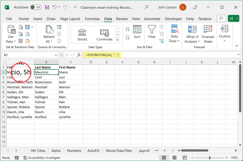
To split the first name in the list located in cell A2 (column A), we need to extract all text before the last occurrence of a “comma-space” character set. The formula would be:
=TEXTBEFORE(A2, “, “)

To split the second name in the list located in cell A2 (column A), we need to extract all text after the last occurrence of a “comma-space” character set. The formula would be:
=TEXTAFTER(A2, “, “)
There are many methods to separate names in Excel using the Convert Text to Columns Wizard, formulas, and the Flash Fill feature available in the Data Tab to make your data more manageable. Check out this tutorial: How to Separate Names in Excel for Cleaner Data by Productivity Portfolio.
Create a List of Sequential Data
You can quickly create a list of dates, in sequential order, by using the Fill Handle ![]() or the Fill command.
or the Fill command.
Use the Fill Handle
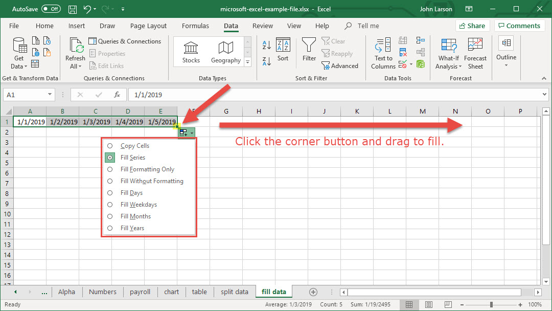
1. Select the cell that contains the first date. Drag the fill handle across the adjacent cells that you want to fill with sequential dates.
2. Select the fill handle at the lower-right corner of the cell, hold down, and drag to fill the rest of the series. Fill handles can be dragged up, down, or across a spreadsheet.
Use the Fill command
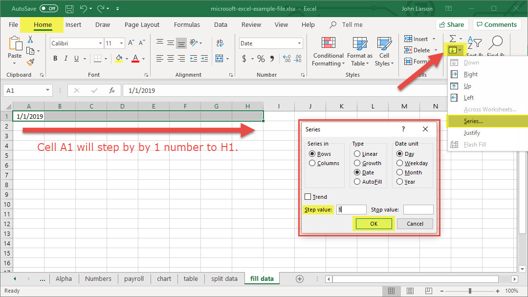
1. Select the cell with the first date. Then select the range of cells you want to fill.
2. Select Home > Editing > Fill > Series > Date unit. Select the unit you want to use.
Tip: You can sort dates much like any other data. By default, dates are sorted from the earliest date to the latest date.
Filter for Unique Values or Remove Duplicate Values
In Excel, there are several ways to filter for unique values—or remove duplicate values:
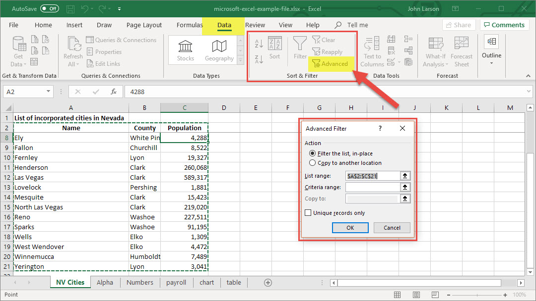
To filter for unique values, click Data > Sort & Filter > Advanced.
![]() You can read more about advanced filtering from Microsoft in this article: Filter by using advanced criteria.
You can read more about advanced filtering from Microsoft in this article: Filter by using advanced criteria.
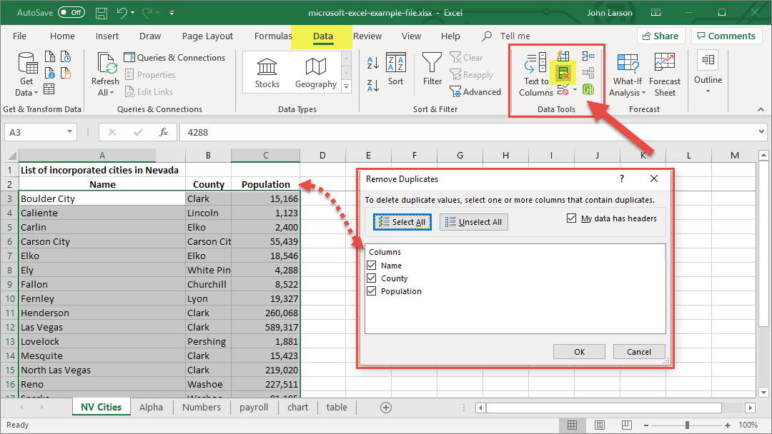
To remove duplicate values, click Data > Data Tools > Remove Duplicates.
To highlight unique or duplicate values, use the Conditional Formatting command in the Style group on the Home tab.
Apply Data Validation to Cells
You can use data validation to restrict the type of data or the values that users enter into a cell. One of the most common data validation uses is to create a drop-down list.
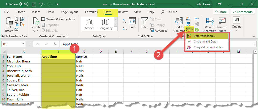
1. Select the cell(s) you want to create a rule for.
2. Select Data >Data Validation.
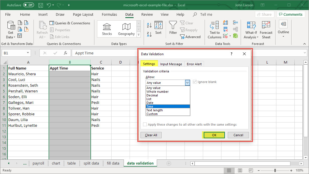
3. On the Settings tab, under Allow, select an option:
- Whole Number – to restrict the cell to accept only whole numbers.
- Decimal – to restrict the cell to accept only decimal numbers.
- List – to pick data from the drop-down list.
- Date – to restrict the cell to accept only date.
- Time – to restrict the cell to accept only time.
- Text Length – to restrict the length of the text.
- Custom – for custom formula.
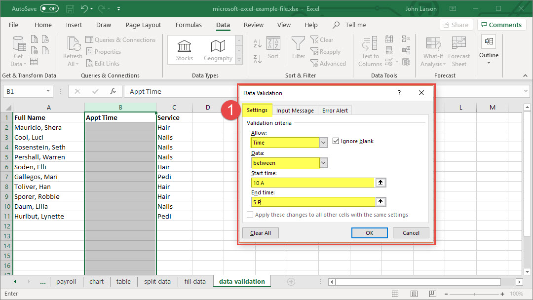
4. Under Data, select a condition:
- between
- not between
- equal to
- not equal to
- greater than
- less than
- greater than or equal to
- less than or equal to
5. On the Settings tab, under Allow, select an option:
6. Set the other required values, based on what you chose for Allow and Data. For example, if you select between, then select the Minimum: and Maximum: values for the cell(s).
7. Select the Ignore blank checkbox if you want to ignore blank spaces.
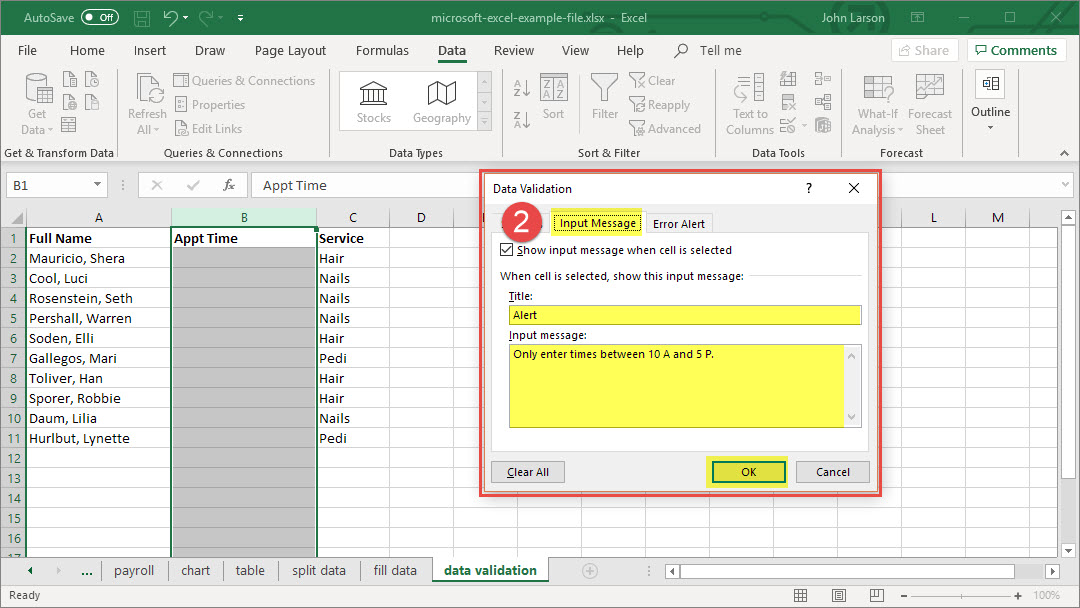
8. If you want to add a Title and message for your rule, select the Input Message tab, and then type a title and input message.
9. Select the Show input message when the cell is selected checkbox to display the message when the user selects or hovers over the selected cell(s).
10. Select OK.
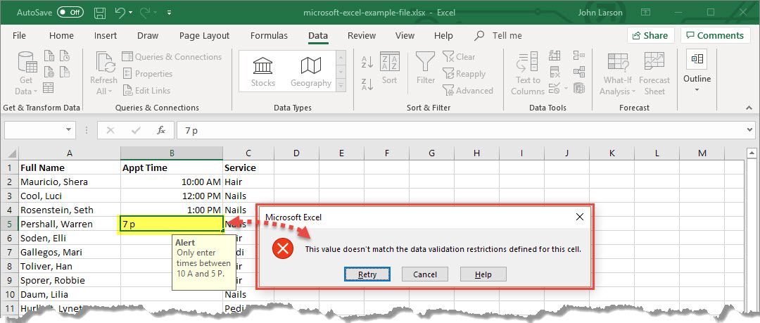
Now, if the user tries to enter a value that is not valid, a pop-up appears with the message, “This value doesn’t match the data validation restrictions for this cell.”
Conditional Formatting
Conditional formatting provides visual cues to help you quickly make sense of your data. For example, it’ll clearly show highs and lows, or other data trends based on the criteria you provide..
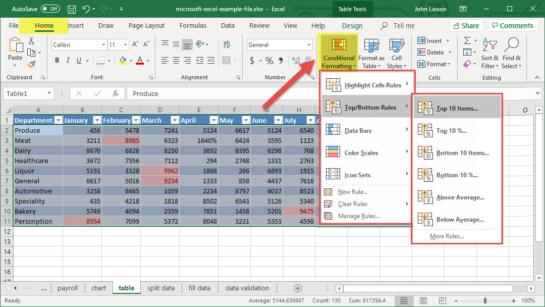
1. Select all the data in a table.
2. Select Conditional Formatting > Top/Bottom Rules > Top 10 Items to see the 10 largest numbers in the table.
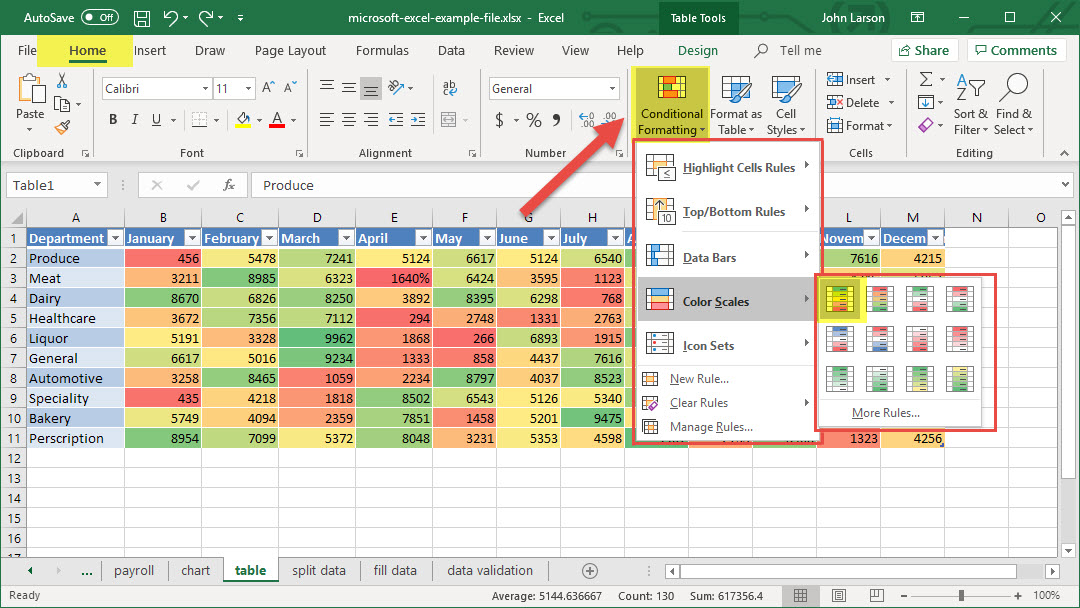
3. Select Conditional Formatting > Data Bars, Color Schemes, or Icon Sets to see how your data can be instantly analyzed. Press Ok when done.