PivotTables

• PivotTable Overview
• Analyze Worksheet Data
• Arrange Fields
• Group or Ungroup Data
• Filter Data
• Data Refresh (Update)
• PivotCharts

Overview

PivotTables are a powerful tool that allows you to summarize, analyze, explore, and present your data in various flexible ways. It enables you to extract the significance from a large, detailed data set by allowing you to rearrange, sort, count, and total or average data stored in one table or spreadsheet.

Pivot Tables are a must-have skill for anyone who regularly works with data in Excel. They provide a straightforward way to turn extensive data into actionable insights without the need for complex formulas or coding skills.

• Sales Reports: Summarize sales data by product, region, or salesperson to identify top performers and best-selling items.
• Financial Analysis: Consolidate financial data to summarize revenues, expenses, and profits by category over different periods.
• Inventory Management: Track inventory levels, reorder times, and categorize stock by various attributes.
• Customer Data Analysis: Segment customers based on purchasing behavior, demographics, or loyalty to tailor marketing strategies.
• Survey Data Analysis: Summarize responses to survey questions, calculate average ratings, and identify patterns or trends in feedback.
• Human Resources: Analyze employee data, including salaries, departmental costs, and performance metrics to inform HR policies.
• Time Tracking: Aggregate timesheet data to calculate total hours worked by project, task, or employee, aiding in project management and payroll.
• Educational Analysis: Assess student performance across various tests and subjects to identify areas of strength and opportunities for improvement.

Download and open the PivotTable spreadsheet to see how to work with the Table and use the examples.

Analyze Worksheet Data

A PivotTable is a powerful tool to calculate, summarize, and analyze data that lets you see comparisons, patterns, and trends in your data.

Create a PivotTable

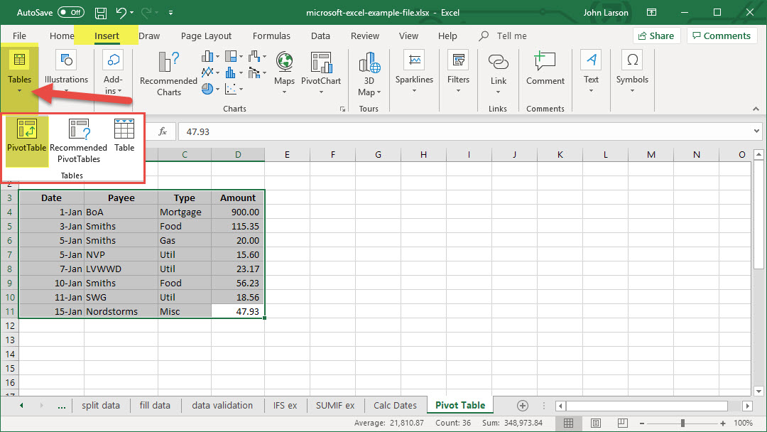
1. Select the cells you want to create a PivotTable from.

Note: Your data shouldn’t have any empty rows or columns. It must have only a single-row heading.

2. Select Insert > PivotTable.

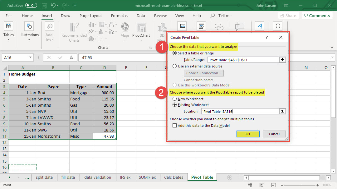
3. Under Choose the data that you want to analyze, select Select a table or range.

4. In Table/Range, verify the cell range.

5. Under Choose where you want the PivotTable report to be placed, select New worksheet to place the PivotTable in a new worksheet or Existing worksheet and then select the location you want the PivotTable to appear.

6. Select OK.

Building out your PivotTable

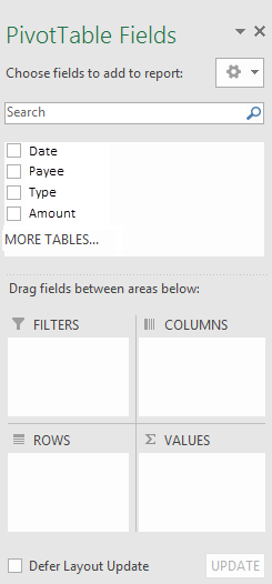
1. To add a field to your PivotTable, select the field name checkbox in the PivotTables Fields pane.

Note: Selected fields are added to their default areas: non-numeric fields are added to Rows, date and time hierarchies are added to Columns, and numeric fields are added to Values.

2. To move a field from one area to another, drag the field to the target area.

Use the Field List to Arrange Fields

After you create a PivotTable, you’ll see the Field List. You can change the design of the PivotTable by adding and arranging its fields.

The Field List should appear when you click anywhere in the PivotTable. If you click inside the PivotTable but don’t see the Field List, open it by:

1. Clicking anywhere in the PivotTable.

2. Then, show the PivotTable Tools on the ribbon and click Analyze> Field List.

The Field List has a field section in which you pick the fields you want to show in your PivotTable, and the Areas section (at the bottom) in which you can arrange those fields the way you want.

Tip: If you want to change how sections are shown in the Field List, click the Tools button Field List Tools button and then pick the layout you want.

Add and rearrange fields in the Field List

Use the field section of the Field List to add fields to your PivotTable, by checking the box next to field names to place those fields in the default area of the Field List.

NOTE: Typically, non-numeric fields are added to the Rows area, numeric fields are added to the Values area, and Online Analytical Processing (OLAP) date and time hierarchies are added to the Columns area.

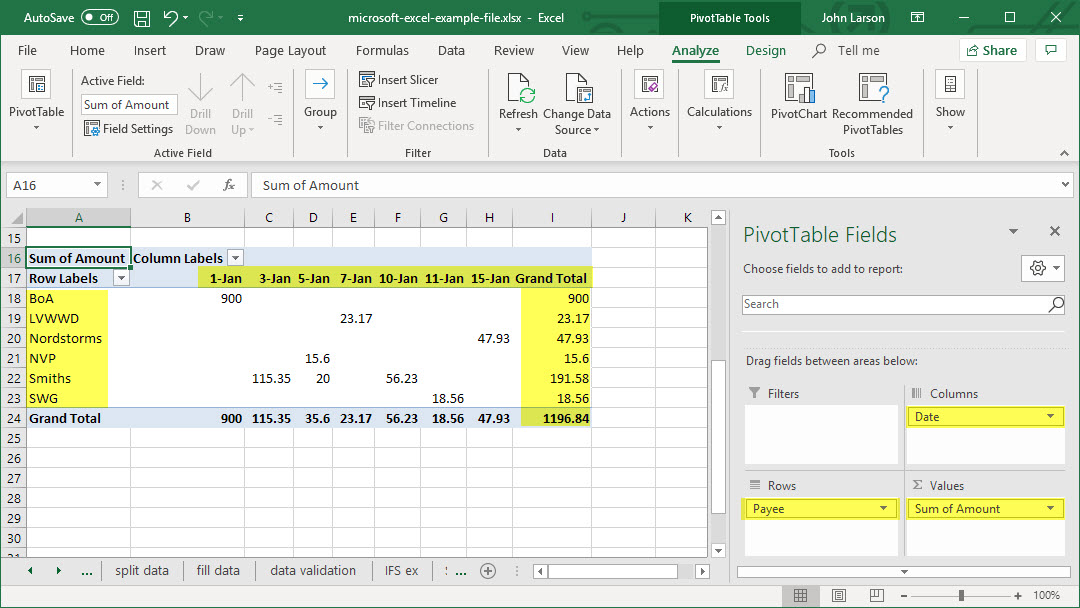
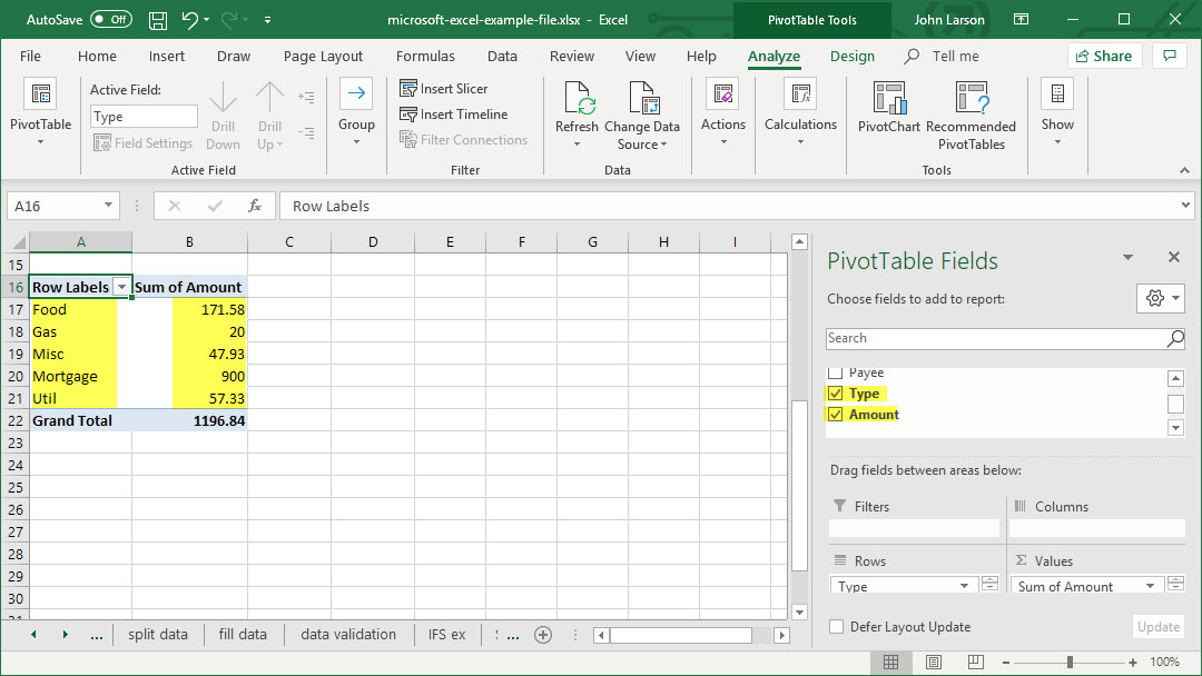
Use the areas section (at the bottom) of the Field List to rearrange fields the way you want by dragging them between the four areas.

Fields that you place in different areas are shown in the PivotTable as follows:

• Filters area fields are shown as top-level report filters above the PivotTable.
• Columns area fields are shown as Column Labels at the top of the PivotTable.
  • Depending on the hierarchy of the fields, columns may be nested inside columns that are higher in position.
• Rows area fields are shown as Row Labels on the left side of the PivotTable.
  • Depending on the hierarchy of the fields, rows may be nested inside rows that are higher in position.
• Values area fields are shown as summarized numeric values in the PivotTable.

Note: If you have more than one field in an area, you can rearrange the order by dragging the fields into the precise position you want. To delete a field from the PivotTable, drag the field out of its areas section.

Group or Ungroup Data

Grouping data in a PivotTable can help you show a subset of data to analyze. For example, you may want to group an unwieldy list of dates or times (date and time fields in the PivotTable) into quarters and months, like this image.

Note: The time grouping feature is new in Excel 2016. With time grouping, relationships across time-related fields are automatically detected and grouped together when you add rows of time fields to your PivotTables. Once grouped together, you can drag the group to your Pivot Table and start your analysis.

Group data

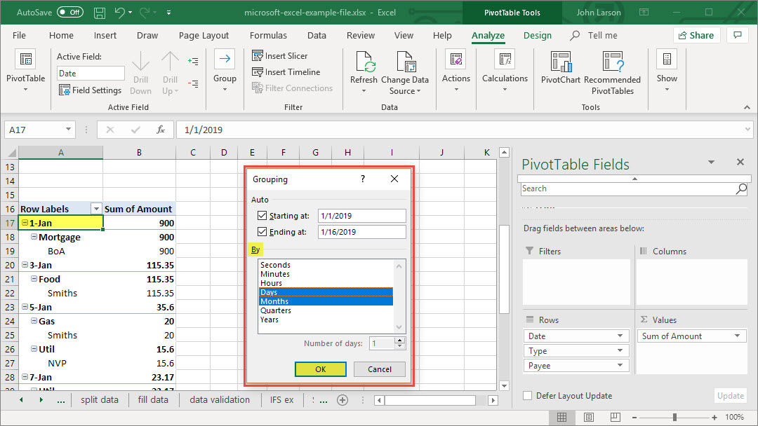
1. In the PivotTable, right-click a value and select Group.

2. In the Grouping box, select Starting at and Ending at checkboxes, and edit the values if needed.

3. Under By, select a time period. For numerical fields, enter a number that specifies the interval for each group.

4. Select OK.

Group selected items

1. Hold Ctrl and select two or more values.

2. Right-click and select Group.

Name a group

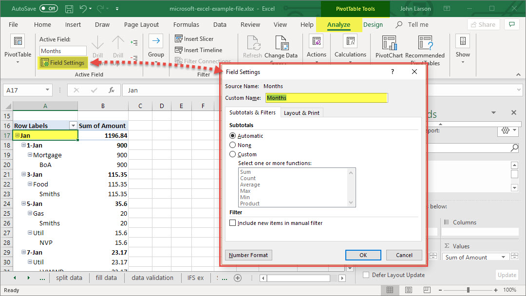
1. Select the group.

2. Select Analyze > Field Settings.

3. Change the Custom Name to something you want and select OK.

Ungroup grouped data

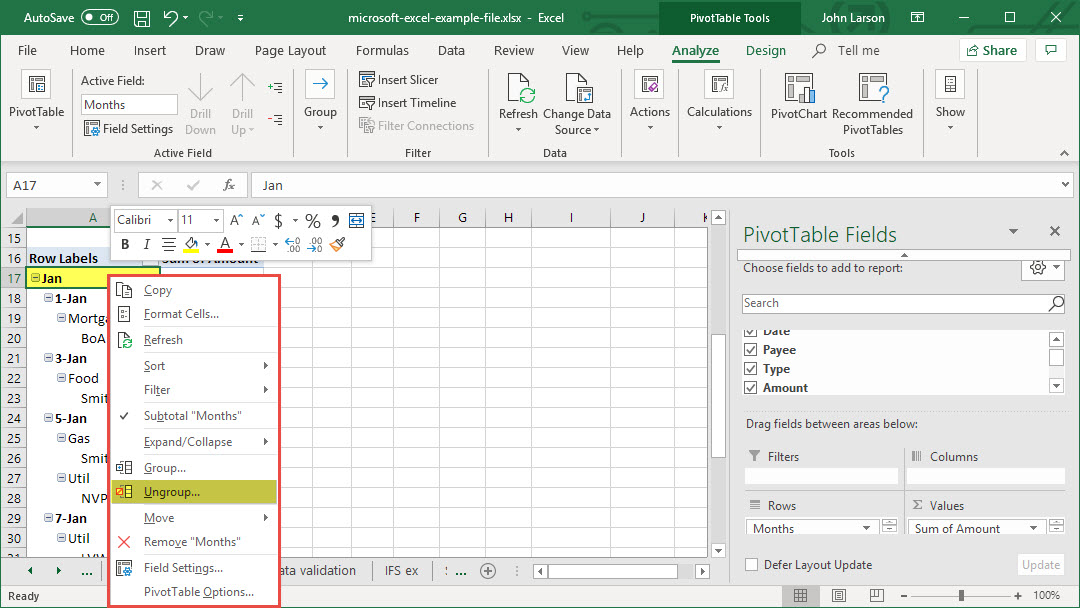
1. Right-click any item that is in the group.

2. Select Ungroup.

Filter Data

Filter your data to focus on a smaller portion of your PivotTable data for in-depth analysis. First, insert one or more slicers for a quick and effective way to filter your data. Slicers have buttons you can click to filter the data, and stay visible with your data, so you always know what fields are shown or hidden in the filtered PivotTable.

Tip: Now in Excel 2016, you can multi-select slicers by clicking the button on the label as shown above.

Filter data in a PivotTable

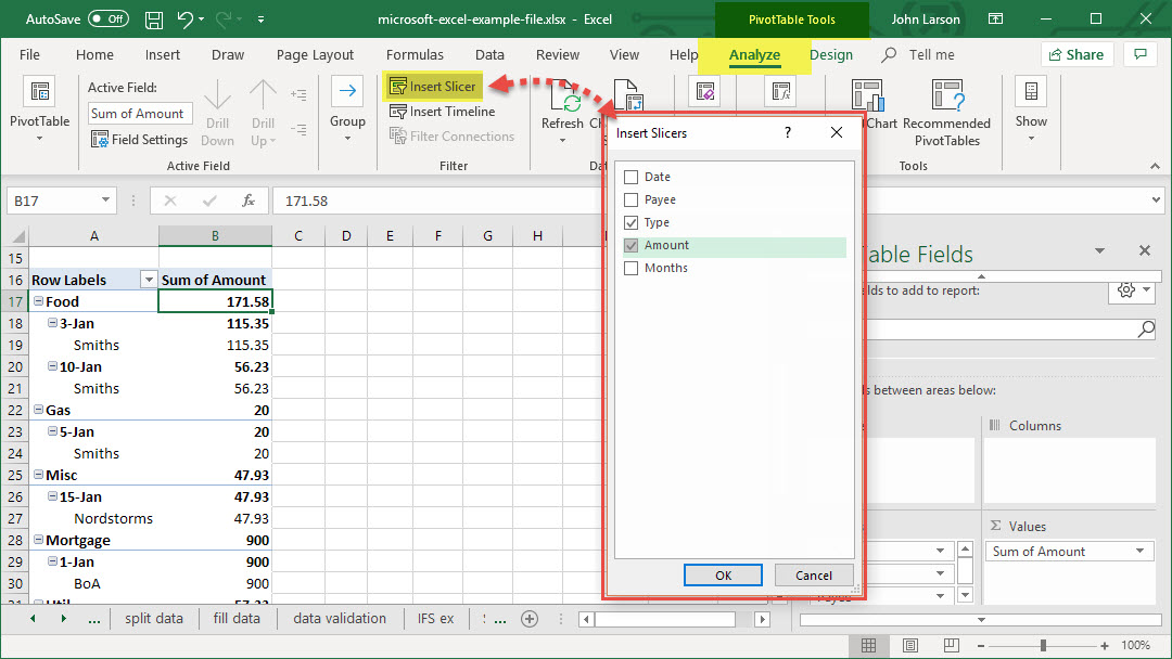
1. Select a cell in the PivotTable. Select Analyze > Insert Slicer .

2. Select the fields you want to create slicers for. Then select OK.

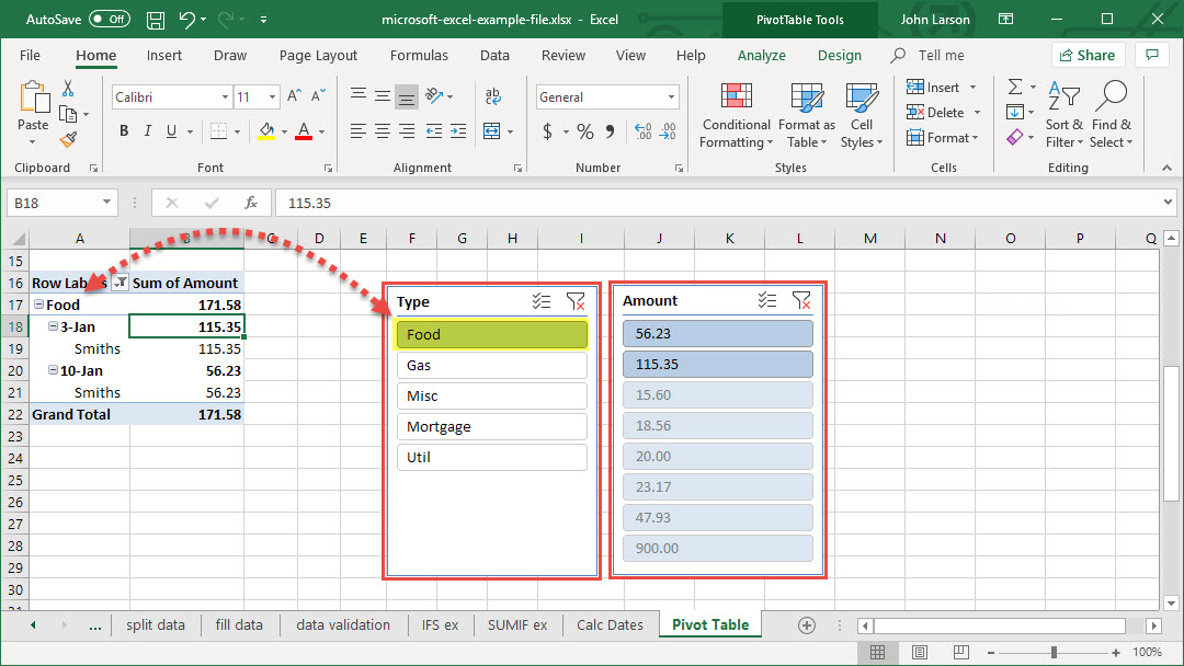
3. Select the items you want to show in the PivotTable.

Filter data manually

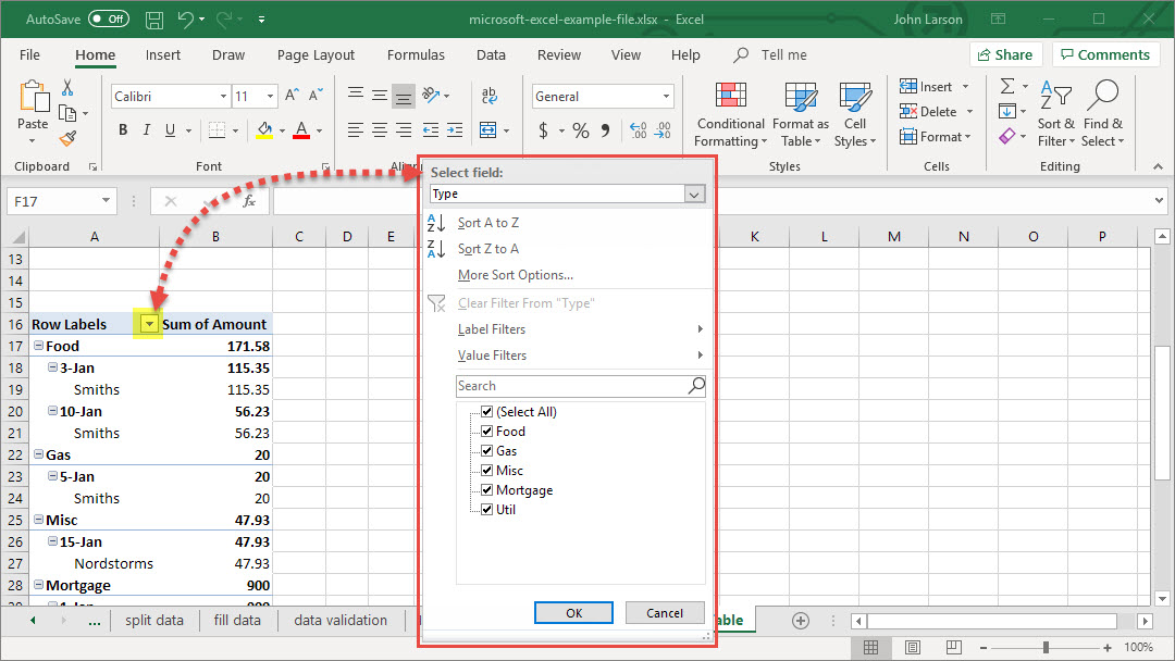
1. Select the column header arrow Filter drop-down arrow for the column you want to filter.

2. Uncheck (Select All) and select the boxes you want to show. Then select OK.

Data Refresh (Update)

PivotTables can be updated with the latest data either automatically or manually.

Automatic

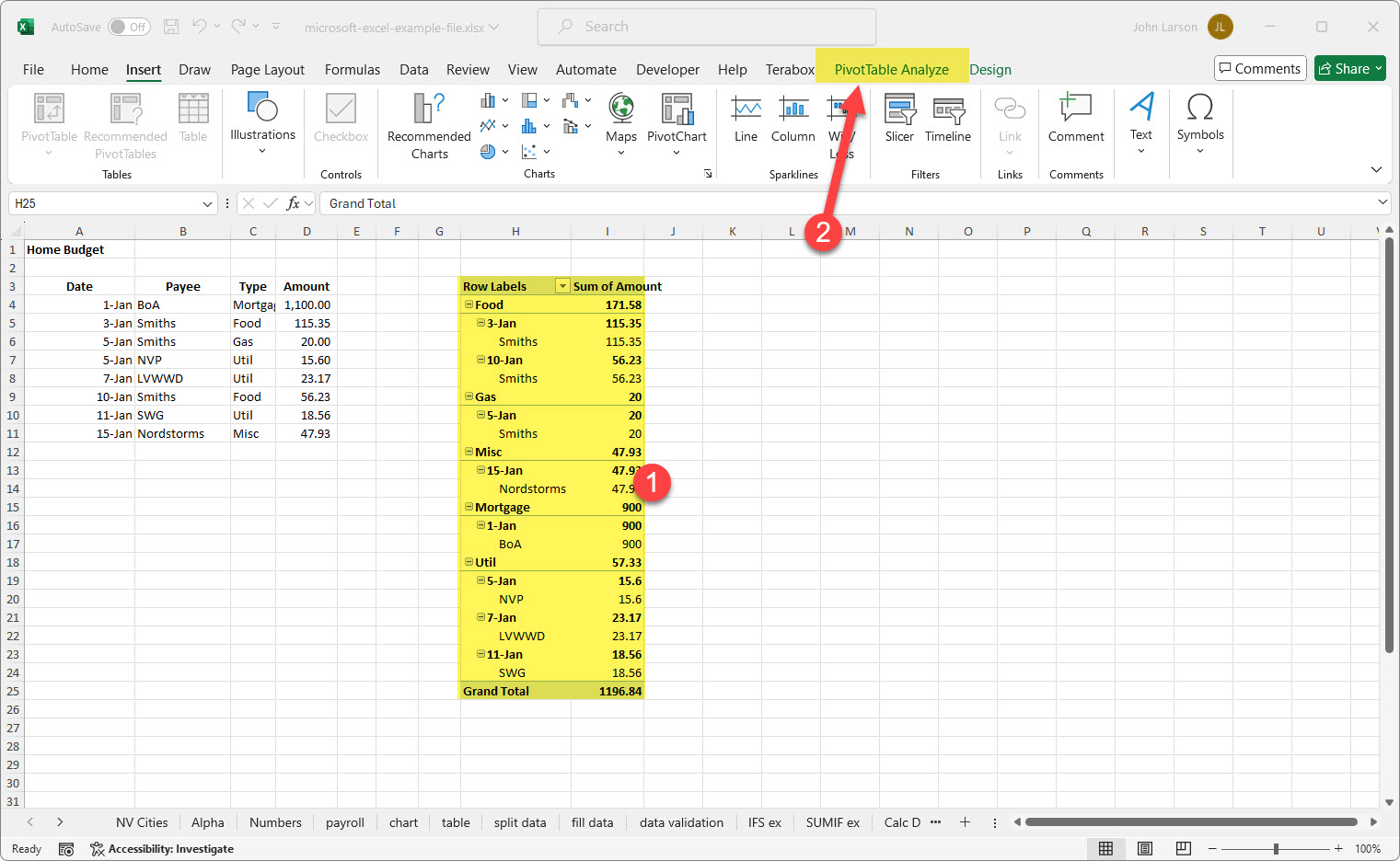
1. Select the 1) PivotTable to show the 2) PivotTable Analyze tab on the ribbon.

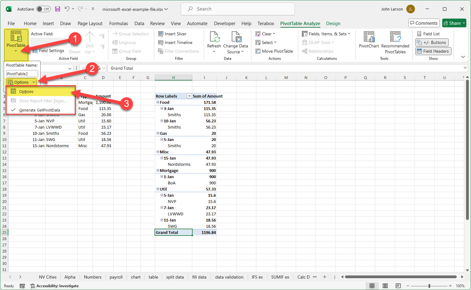
2. Select 1) PivotTable Options dropdown, 2) Options dropdown, 3) Options button.

 

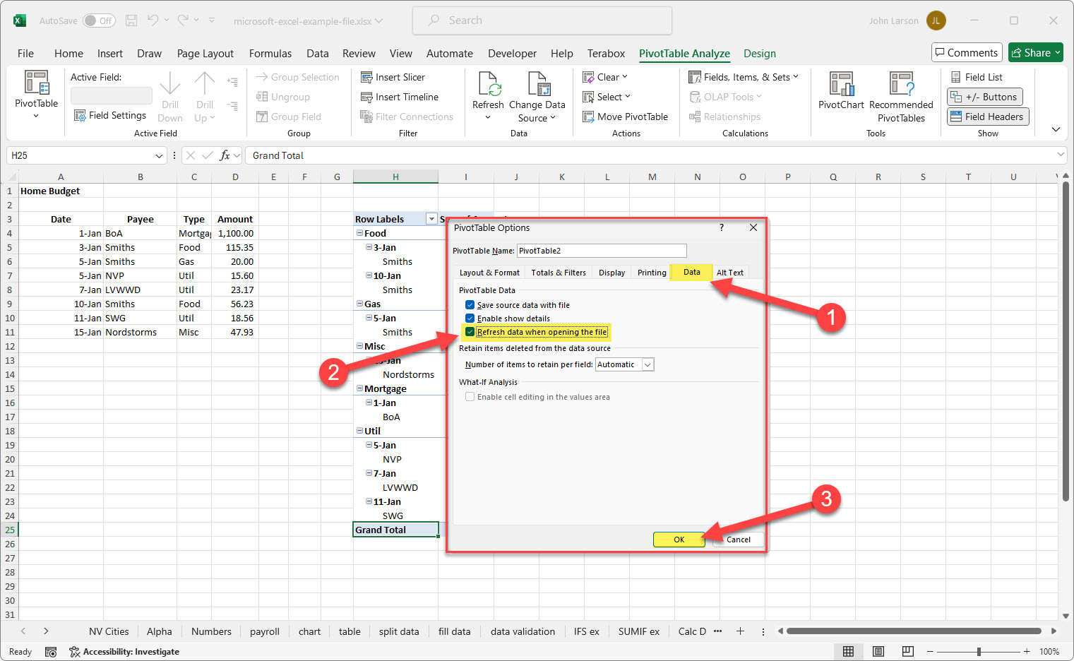
3. Select the 1) Data tab, 2) check the Refresh data when opening the file box, then 3) OK.

4. Your PivotTable will now refresh every time you option the worksheet.

Manually

1. Select the 1) PivotTable to show the 2) PivotTable Analyze tab on the ribbon.

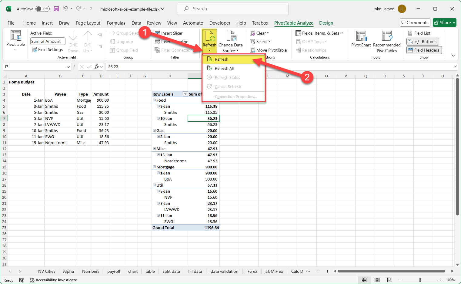
1. 1) Select PivotTable Refresh dropdown, 2) click the Refresh button to update the data group, or press Alt+F5.

• This will update the PivotTable you’ve selected. To update all of the PivotTables in your worksheet, select the Refresh All button.
• If refreshing takes longer than expected, on the PivotTable Analyze tab, select the Refresh arrow and choose Refresh Status to check the refresh status.
• To stop refreshing, select Cancel Refresh.

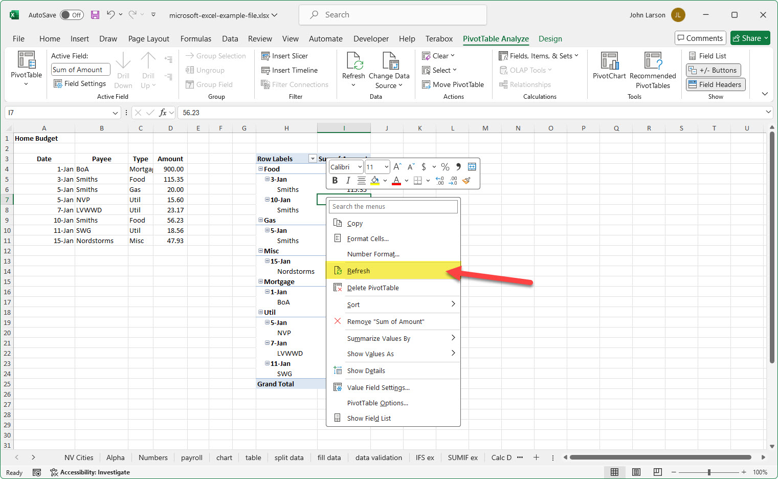
Tip: You can right-click the PivotTable and select Refresh to update the selected PivotTable.

PivotChart

Sometimes it’s hard to see the big picture when your raw data hasn’t been summarized. Your first instinct may be to create a PivotTable, but not everyone can look at numbers in a table and quickly see what’s going on. PivotCharts are a great way to add data visualizations to your data.

Create a PivotChart

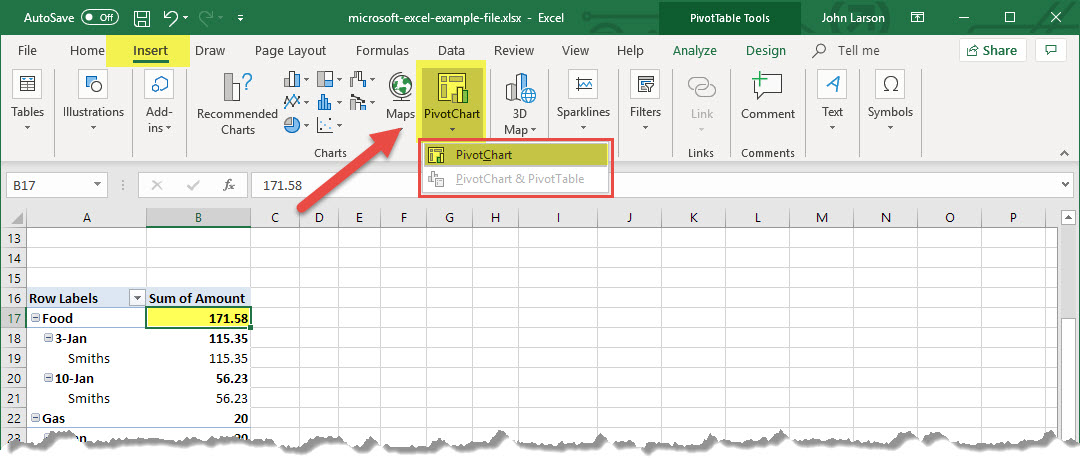
1. Select a cell in your table.

2. Select Insert > PivotChart option on the ribbon .

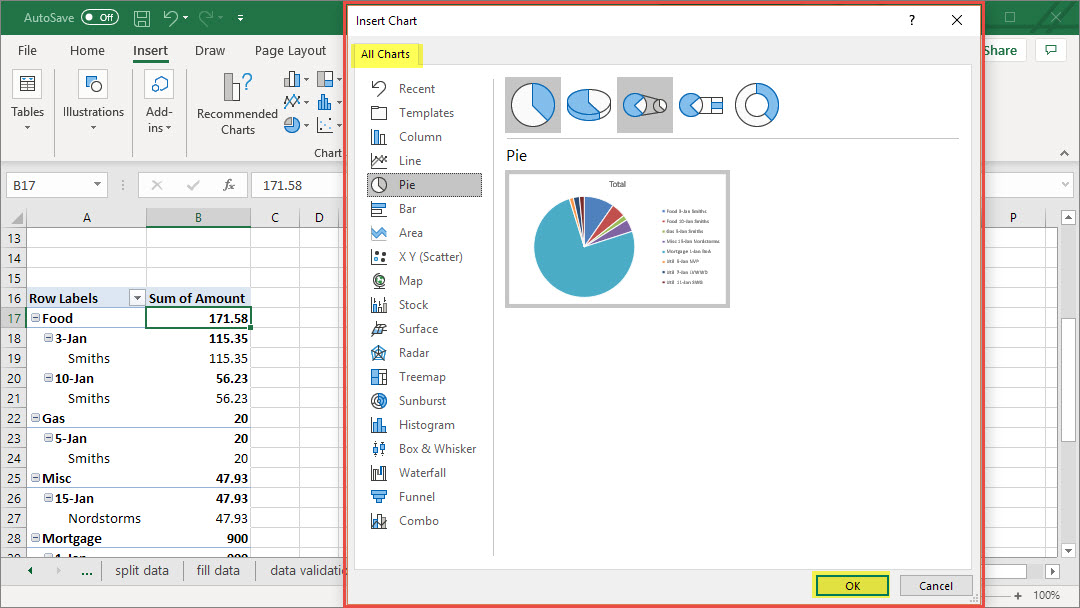
3. Select a chart.

4. Select OK.

Create a chart from a PivotTable

1. Select a cell in your table.

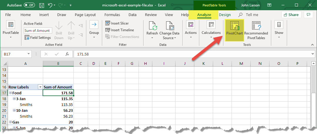
2. Select PivotTable Tools > Analyze > PivotChart option on the ribbon .

3. Select a chart.

4. Select OK.