Cells Overview
It’s essential to understand cells and cell content in Excel to be able to use it to calculate, analyze, and organize data. In this lesson, you will learn how to select cells, insert content, and delete cells and cell content. You will also learn how to cut, copy and paste cells, drag and drop cells, and fill cells using fill data.
Cells are the basic building blocks of a worksheet. Cells can contain a variety of content such as text, formatting attributes, formulas and functions. To work with cells, you’ll need to know how to select them, insert content, and delete cells and cells content.
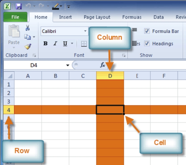
Each rectangle in a worksheet is called a cell. A cell is the intersection of a row and a column.
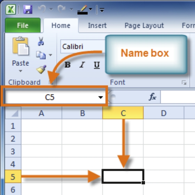
Each cell has a name, or a cell address based on which column and row it intersects. The cell address of a selected cell appears in the Name Box. In the example above, you can see that C5 is selected.
You can also select multiple cells at the same time. A group of cells is known as a cell range. Rather than a single cell address, you will refer to a cell range using a cell addresses of the first and last self in the sell range separated by a colon. For example, a cell range that included cells A1, A2, A3, A4 and 85 would be written as A1:A5.
To Select a Cell:
1. Click on a cell to select it. When a cell is selected you will notice that the borders of the cell appear bold and the column heading and row heading of the cell are highlighted.
2. Release your mouse. The cell will stay selected until you click on another cell in the worksheet.
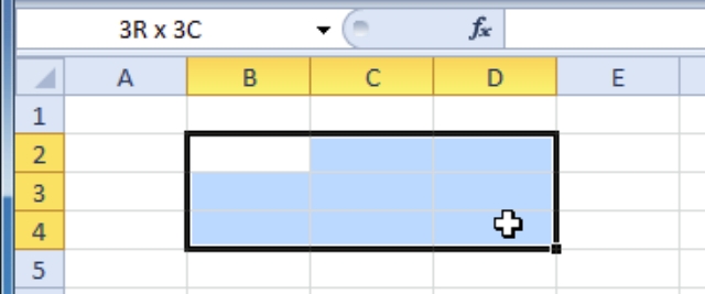
To Select Multiple Cells:
1. Click and drag your mouse until all of the adjoining cells you want are highlighted.
2. Release your mouse. The cells will stay selected until you click on another cell in the worksheet.
Cell Content
Each cell can contain its own text, formatting, comments, formulas, and functions:
- Text: Cells can contain letters, numbers, and dates.
- Formatting attributes: Cells can contain formatting attributes that change the way letters, numbers, and dates are displayed. For example, dates can be formatted as MM/DD/YYYY or Month/D/YYYY.
- Comments: Cells can contain comments from multiple reviewers.
- Formulas and Functions: Cells can contain formulas and functions that calculate cell values. For example, SUM(cell 1, cell 2…) is a formula that can add the values in multiple cells.
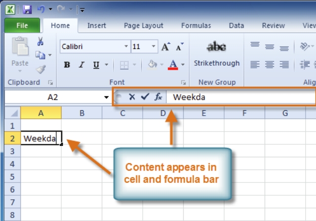
To Insert Content:
1. Click on a cell to select it.
2. Enter content into the selected cell using your keyboard. The content appears in the cell and in the formula bar. You also can enter or edit cell content from the formula bar.

To Delete Content Within Cells:
1. Select the cells which contain content you want to delete.
2. Click the Clear command on the ribbon. A dialog box will appear.
3. Select Clear Contents.
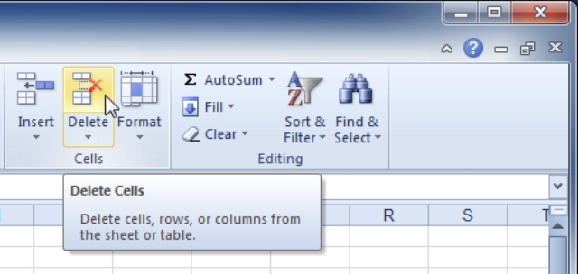
To Delete Cells:
1. Select the cells that you want to delete.
2. Choose the Delete command from the ribbon
There is an important difference between deleting the content of a cell and deleting the cell itself. If you delete the cell, by default the cells around the deleted cell(s) will shift to fill the deleted area.
To Copy and Paste Cell Content:
1. Select the cells you wish to copy.
2. Click the Copy command. The border of the selected cells will change appearance.
3. Select the cell or cells where you want to paste the content.
4. Click the Paste command. The copied content will be entered into the highlighted cells.
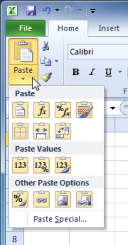
To Access More Paste Options:
There are more Paste options that you can access from the drop-down menu on the Paste command. These options may be convenient to advanced users who are working with cells that contain formulas or formatting.
Move or Copy Cells and Cell Contents
Use Cut, Copy, and Paste to move or copy cell contents. Or copy specific contents or attributes from the cells. For example, copy the resulting value of a formula without copying the formula, or copy only the formula.
When you move or copy a cell, Excel moves or copies the cell, including formulas and their resulting values, cell formats, and comments.
You can move cells in Excel by drag and dropping or using the Cut and Paste commands.
Move cells by dragging and dropping
1. Select the cells or range of cells that you want to move or copy.
2. Point to the border of the selection.
3. When the pointer becomes a move pointer ![]() move pointer , drag the cell or range of cells to another location.
move pointer , drag the cell or range of cells to another location.
Move cells by using Cut and Paste
1. Select a cell or a cell range.
2. Select Home > Cut ![]() or press Ctrl+X.
or press Ctrl+X.
3. Select a cell where you want to move the data.
4. Select Home > Paste ![]() or press Ctrl+V.
or press Ctrl+V.
Copy cells by using Copy and Paste
1. Select the cell or range of cells.
2. Select Copy or press Ctrl+C.
3. Select Paste or press Ctrl+V.
Formatting Cells
Appearance
Cells can be formatted to change the size, color, alignment, and font type.
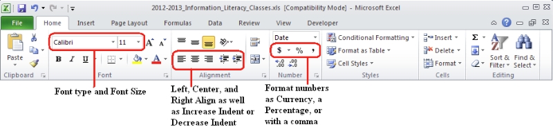
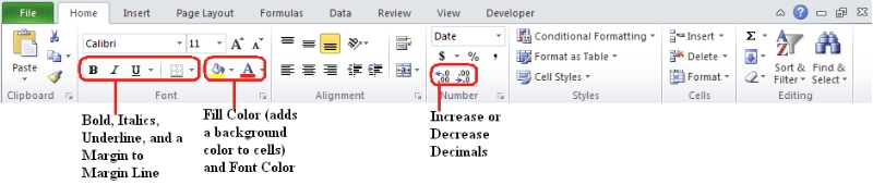
Formatting Cells using the Ribbon
1. Access Formatting using the Ribbon1.Select the cells you want to format.
2. Click the appropriate format button.
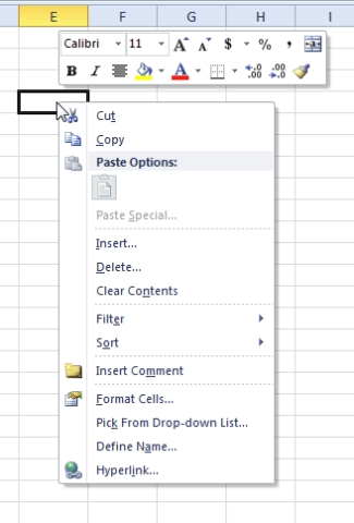
Access Formatting Commands by Right-Clicking:
1. Select the cells you want to format.
2. Right-click on the selected cells. A dialog box will appear where you can easily access many commands that are on the ribbon.
Align or Rotate Text in a Cell
You can change data appearance in a cell by rotating the font angle or changing the data alignment.
Align a column or row
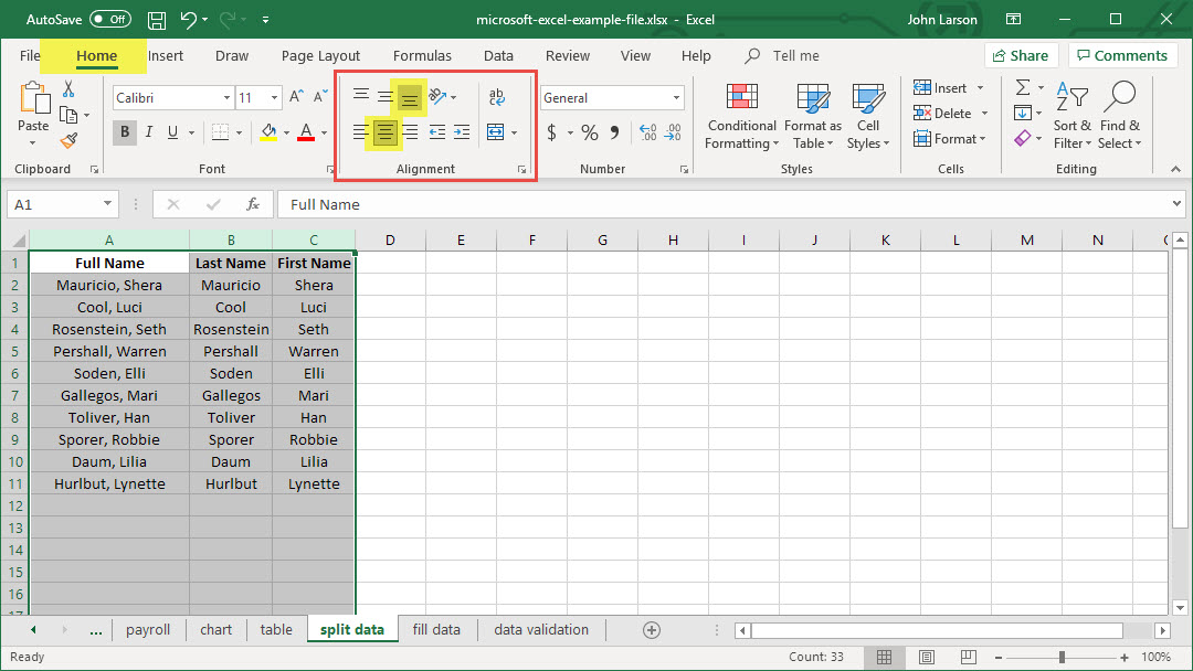
1. Select a column or row.
2. Select Align Left, Center, or Align Right.
3. Select Top Align, Middle Align, or Bottom Align.
Align cells in a workbook
1. Click a cell, or press Ctrl + A to select all cells.
2. Select Align Left, Center, or Align Right.
3. Select Top Align, Middle Align, or Bottom Align.
Rotate text
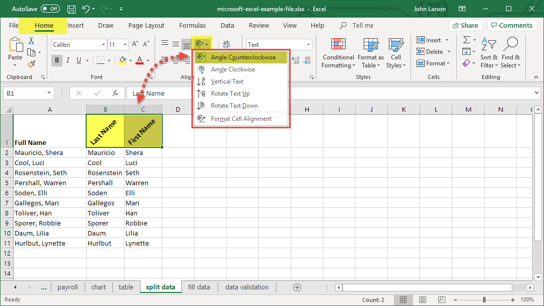
1. Select a cell, row, column, or range.
2. Click Orientation, and then select an option.
You can rotate your text up, down, clockwise, or counterclockwise, or align text vertically.
Numbers
Cells can also be formatted as numbers: currency, percentages, decimals, dates, phone numbers, or social security numbers.
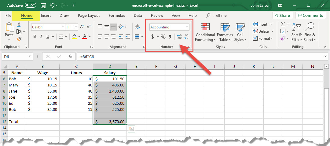
1. Select a cell or a cell range.
2. On the Home tab, select Number from the drop-down or, you can choose one of these options:
- Press Ctrl+1 and select Number.
- Right-click the cell or cell range, select Format Cells…, and select Number.
- Select the dialog box launcher Alignment Settings next to Number Dialog box launcher and then select Number.
3. Select the format you want.
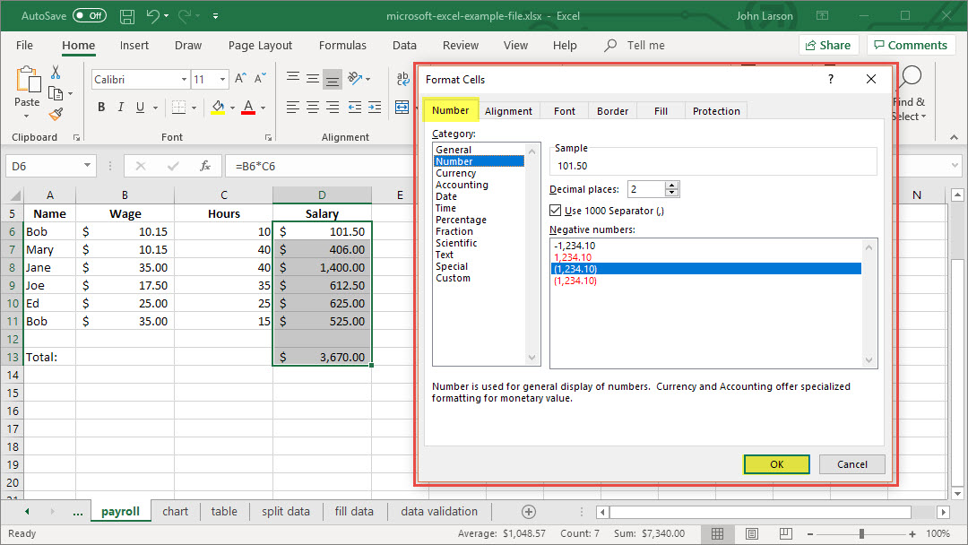
Number formats
To see all available number formats, click the Dialog Box Launcher next to Number on the Home tab in the Number group.
| Format | Description |
| General | The default number format that Excel applies when you type a number. For the most part, numbers that are formatted with the General format are displayed just the way you type them. However, if the cell is not wide enough to show the entire number, the General format rounds the numbers with decimals. The General number format also uses scientific (exponential) notation for large numbers (12 or more digits). |
| Number | Used for the general display of numbers. You can specify the number of decimal places that you want to use, whether you want to use a thousands’ separator, and how you want to display negative numbers. |
| Currency | Used for general monetary values and displays the default currency symbol with numbers. You can specify the number of decimal places that you want to use, whether you want to use a thousands’ separator, and how you want to display negative numbers. |
| Accounting | Also used for monetary values, but it aligns the currency symbols and decimal points of numbers in a column. |
| Date | Displays date and time serial numbers as date values, according to the type and locale (location) that you specify. Date formats that begin with an asterisk (*) respond to changes in regional date and time settings that are specified in the Control Panel. Formats without an asterisk are not affected by Control Panel settings. |
| Time | Displays date and time serial numbers as time values, according to the type and locale (location) that you specify. Time formats that begin with an asterisk (*) respond to changes in regional date and time settings that are specified in the Control Panel. Formats without an asterisk are not affected by Control Panel settings. |
| Percentage | Multiplies the cell value by 100 and displays the result with a percent (%) symbol. You can specify the number of decimal places that you want to use. |
| Fraction | Displays a number as a fraction, according to the type of fraction that you specify. |
| Scientific | Displays a number in exponential notation, replacing part of the number with E+n, where E (which stands for Exponent) multiplies the preceding number by 10 to the nth power. For example, a 2-decimal Scientific format displays 12345678901 as 1.23E+10, which is 1.23 times 10 to the 10th power. You can specify the number of decimal places that you want to use. |
| Text | Treats the content of a cell as text and displays the content exactly as you type it, even when you type numbers. |
| Special | Displays a number as a postal code (ZIP Code), phone number, or Social Security number. |
| Custom | Allows you to modify a copy of an existing number format code. Use this format to create a custom number format that is added to the list of number format codes. You can add between 200 and 250 custom number formats, depending on the language version of Excel that is installed on your computer. |
Custom numbers
You can create and build custom numeric formats to show your numbers as percentages, currency, dates, etc.
To create a custom number format, you start by selecting one of the built-in number formats as a starting point. You can then change any one of the code sections of that format to create your custom number format.
A number format can have up to four sections of code, separated by semicolons. These code sections define the format for positive numbers, negative numbers, zero values, and text, in that order.
<POSITIVE>;<NEGATIVE>;<ZERO>;<TEXT>
For example, you can use these code sections to create the following custom format:
[Blue]#,##0.00_);[Red](#,##0.00);0.00;”sales “@
You do not have to include all code sections in your custom number format. If you specify only two code sections for your custom number format, the first section is used for positive numbers and zeros, and the second section is used for negative numbers. If you specify only one code section, it is used for all numbers. If you want to skip a code section and include a code section that follows it, you must include the ending semicolon for the section that you skip.
1. Select the numeric data.
2. Select More in the Number group.
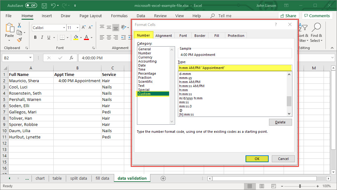
3. Select Custom.
4. In the Type list, select an existing format, or type a new one in the box.
5. To add text to your number format:
- Type what you want in quotation marks.
- Add a space to separate the number and text.
6. Select OK.
Merge and Unmerge Cells
You can’t split an individual cell, but you can make it appear as if a cell has been split by merging the cells above it.
Merge cells
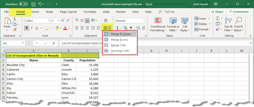
1. Select the cells to merge.
2. Select Merge & Center.
Important: When you merge multiple cells, the contents of only one cell (the upper-left cell for left-to-right languages, or the upper-right cell for right-to-left languages) appear in the merged cell. The contents of the other cells that you merge are deleted.
Unmerge cells
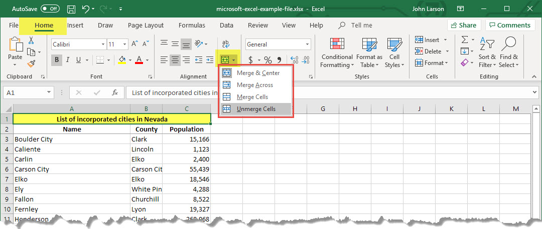
1. Select the Merge & Center down arrow.
2. Select Unmerge Cells.
Important:
- You cannot split an unmerged cell. If you are looking for information about how to split the contents of an unmerged cell across multiple cells.
- After merging cells, you can split a merged cell into separate cells again. If you don’t remember where you have merged cells, you can use the Find command to quickly locate merged cells.